Change Detection

arcgispro

geospatial

map

esri

In this project, we will solve another common GIS problem: determining which areas are changing in times. With rapidly developing remote sensing imagery, it is useful in detecting changes in features on the surface of the Earth. To detect changes in land use and land cover, imagery is required, usually from the same sensor and from two different dates. The interval between times can be as short as a few days (e.g. detect impacts of natural disasters), a few mouths (e.g. detect growth in large agricultural fields) or a few to several years (e.g. changes in forest extent).

The ability to find changes that occur in remote sensing images, this method can be applied in real applications such as:

1. Land use changes (conversion from forest to urban)
2. Expanding urban areas (urban to urban comparison)
3. Effects of natural disasters (such as hurricanes and wildland fires)
4. Impacts of insect infestations on forest cover.
5. etc.

Change detection means applying image differencing, subtracting corresponding pixel values at each pixel, and then displaying the differences as colors, so the areas that differ in brightness can be easily identified. Change detection applies algorithms specifically designed to detect meaningful changes, in contrast to image differences originating in ephemeral (or superficial) features that do not signify meaningful differences over time.

A critical first step in a change detection analysis is identifying and selecting suitable pairs of images acquired over the same region.

1. The two images must register either to each other or to the surface of the Earth—the region they cover must match exactly when superimposed.
2. The images must be acquired during the same season to track long-term changes, such as deforestation.
3. It is vital that no significant atmospheric effects have impacted an image.
4. The two images must be compatible in almost every respect, including but not limited to scale, geometry, and resolution. Otherwise, the change detection algorithm interprets incidental differences in image characteristics as genuine landscape changes.

Many alternative change detection algorithms exist and have been evaluated. Two main change detection approaches are pre-classification and post-classification.

1. Pre-classification change detection examines differences in two images before any classification process.
2. Post-classification change detection defines changes by comparing pixels in a pair of classified images in which pixels have already been assigned to classes. Post-classification change detection typically reports changes as a summary, a difference in digital numbers, of the from-to changes of categories between two dates.

For more details, custom and robust algorithms for Change Detection we can visit this page.

Study case scenario

On June 1, 2018, a fire started in the San Juan National Forest of southwest Colorado. The cause of the fire remains unknown. This fire was named the “416 Fire”. As of June 21, 2018, the fire had destroyed over 34,000 acres of forest and was only 35% contained. The extensive nature of the fire, and the inability to contain it, was directly related to recent drought conditions in Colorado.

NOAA had deemed this region to be in an exceptional drought. A typical annual snowfall for this region is approximately 71 inches. However, in the 2017/2018 winter season, snowfall was 65% less than average. Local snowpack, typically present in June, was gone by June 2018.

Workflows

We will do the change detection results produced using two other methods— Raster Functions and Raster Calculator.

1. Raster Functions — in this part, we will use Change Detection Wizard tool from ArcGIS Pro. This tool has 3 types of change detection method to give more broad workflows:
   • Categorical change — Identify the type of change that has occurred between two thematic or categorical rasters, such as land cover. You can save your final output as a raster dataset, a polygon feature class, or a raster function template.
   • Pixel value change — Calculate the difference in pixel values between two continuous rasters, such as temperature rasters or multiband imagery. You can save your final output as a raster dataset, a polygon feature class, or a raster function template.
   • Spectral change detection — Calculate the spectral difference between two multiband rasters by treating each pixel spectra as a vector. You can save your final output as a raster dataset, a polygon feature class, or a raster function template.
   • Time series change — Identify the date of change in a time series of images using either the Continuous Change Detection and Classification (CCDC) method or the Landsat-based Detection of Trends in Disturbance and Recovery (LandTrendr) method. You can extract the date of earliest, latest, or largest change, or the total number of changes on a pixel-by-pixel basis.
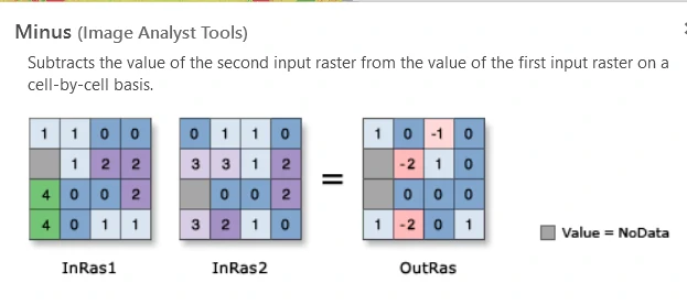
2. Raster Calculator — in this part, we will use a simple yet quite powerful process to calculate difference value in raster. By utilize Minus tools under Image Analyst Tools, we can subtracts the value of the two inputs raster on a cell-by-cell basis.

The Dataset

To analyze change detection from above scenario, we can get dataset from Earth Explore to get Lansat 8 images. We need two Landsat images (Landsat 8) for this region before proceeding. The images are WRS2 type, Path 35, and Row 34, with June 15, 2017, and June 18, 2018 dates.

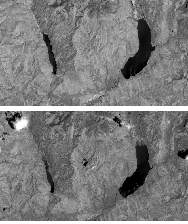
The two images needed are identified in image below, the lack of snow cover is evident in the June 18, 2018, image compared to the June 15, 2017, image (white circle).

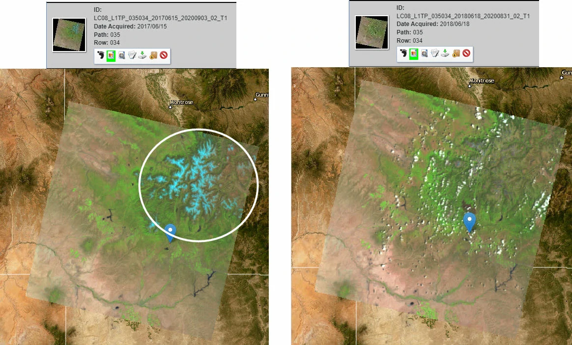
In this project, we need only Band 5 - near infrared(NIR) for each date to get more detail about changes due to the fire’s impact on vegetation. A fire will significantly lower biomass. We will use Band 5 because in the near infrared, emphasizes biomass content and supports the identification of shorelines. Shorelines discriminate between land and water, drought changes water body size, thus changing shorelines, and snow is just frozen water—all pertinent to our study. With downside for Band 5 that this band will experience little atmostpheric scattering.

June 15, 2017

June 18, 2018

The Change Detection Process

ArcGIS Pro provides multiple methods to conduct change detection. This project will show a step-by-step change detection method. Then, we will give the change detection results produced using two other methods — Raster Functions and Raster Calculator.

Raster Functions

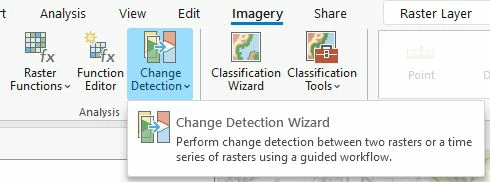
In this part, we use Change Detection Wizard tool from ArcGIS Pro. To access this tool, go under the Imagery tab, locate Change Detection.

By this tool we will set parameters as follow:

• Change Detection Method = Pixel Value Change (to compute absolute or relative change)
• From Raster = dataset at June 15, 2017
• To Raster = dataset at June 18, 2018
• Processing Extent = Full extent
• Statistics & Histogram Computation (X skip and Y skip) = 10
• Difference type = Absolute
• Band Difference Method = Single Band Difference (Our analysis uses single bands)
• From and To Raster band = 1 - Band_1
• Cell Size Type = Max of
• Extent Type = Intersection of

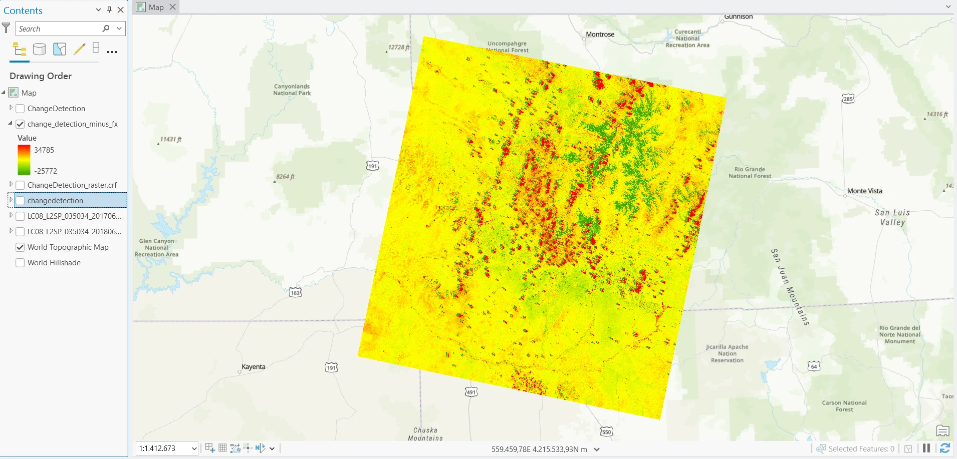
The Result

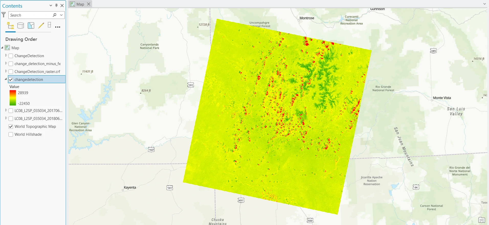
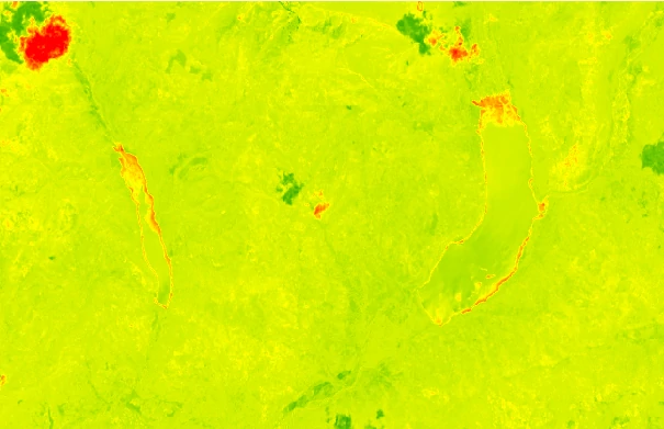
The default symbology represents an increase in a pixel’s digital number. Red is an increase; Green means a decrease, and yellow means little or no change.

The June 18, 2018, image has clouds, and the June 15, 2017, image was cloud-free. The clouds are shown as red, one of the extremes in the change. When performing change detection, we recommend eliminating clouds. Change detection is used to monitor changes in the surface of the Earth. Clouds interfere with that process. For this exercise, the presence versus absence of clouds provides an excellent example of the change detection process.

Another feature that present is, the snow was present in the mountains on June 15, 2017, but no snow was present in the June 18, 2018 image.

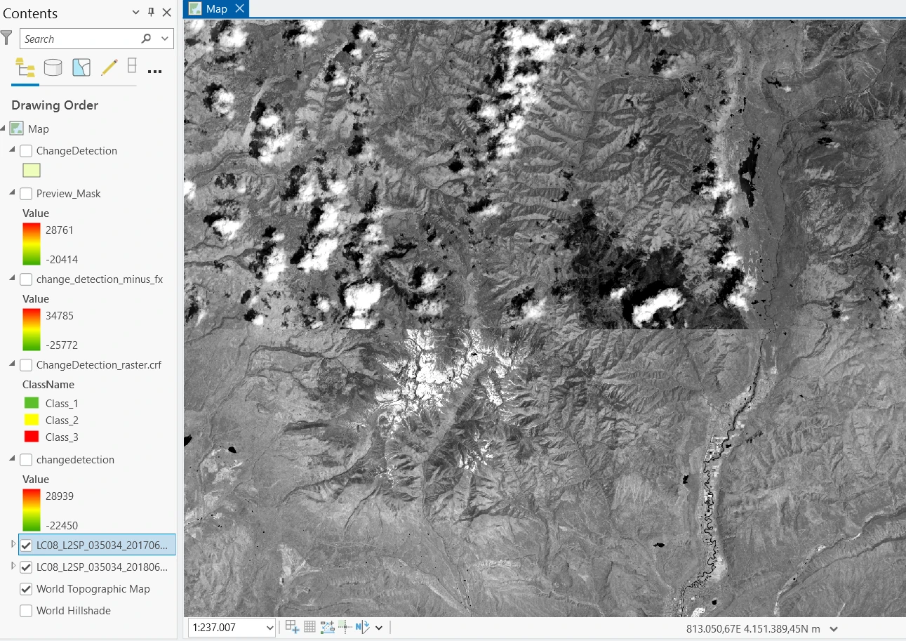
The lack of snow cover from the drought, and the lack of vegetation from the fire, both show a huge change in spectral values. Turn off the image created from the change detection, and let’s look at one more area of change; just to the east of the 416 Wildfire are two lakes.

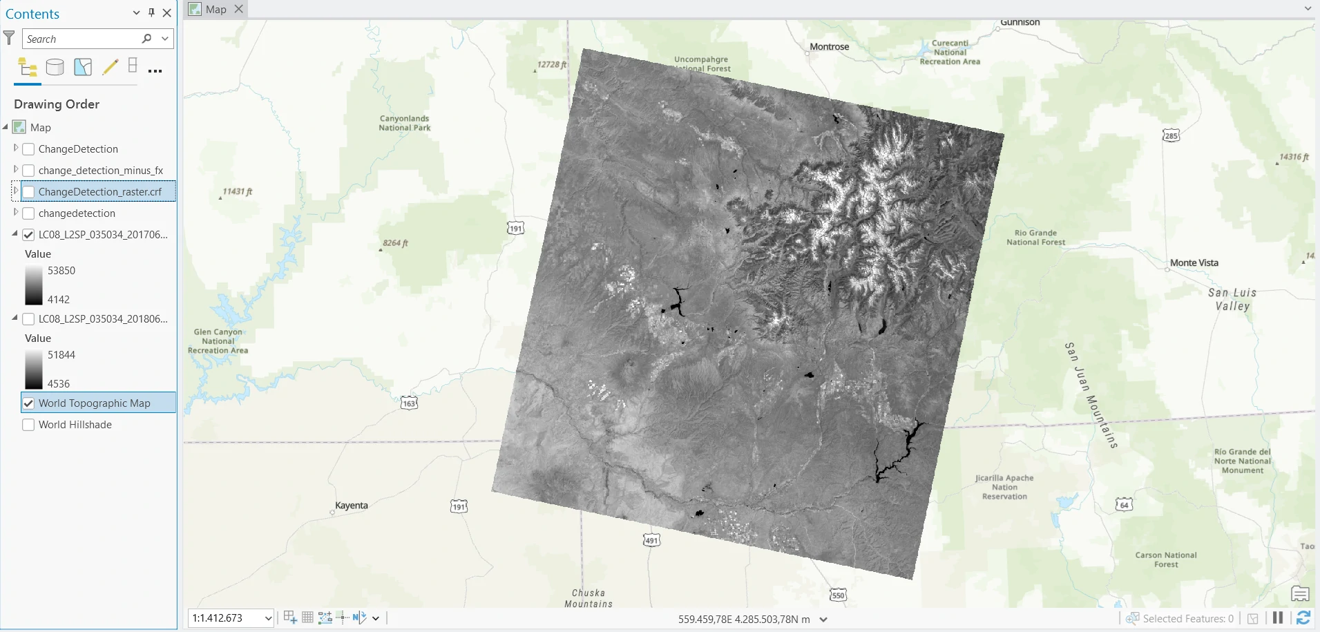
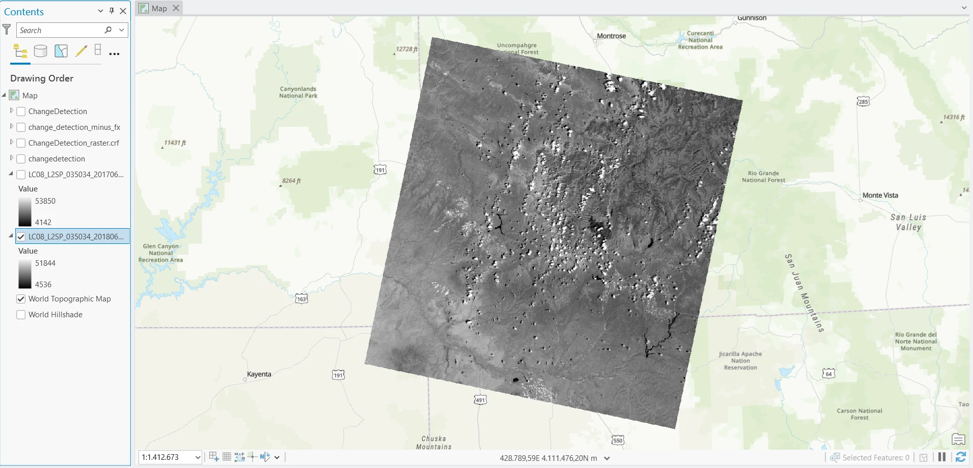
The changes in the black and white images in image above, the original bands, are challenging to see. We are looking at the edges of the two lakes. Look at the edges of the two lakes. The changes are noted in red, again, one of the extremes for the change in spectral values.

The lakes in the June 18, 2018, image are smaller than the earlier June 15, 2017, image. Further, the shallow water in 2018 exposed sediment deposits concealed below the surface in 2017, as indicated by the green areas within the lakes. Also, remember that Band 5 is often used to discern shorelines.

Classification

We can make a clasification to get more easier to get information and make a decision. For that, we can constain our data in histogram (in image below).

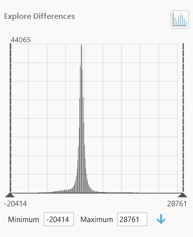
For example we classified the data into 3 values:

• class 1 - [-20414 — -1054.88]
• class 2 - [-1054.88 — 923.43]
• class 3 - [923.43 — 28761]

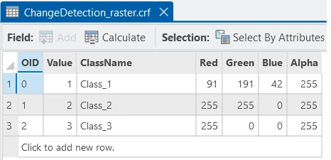
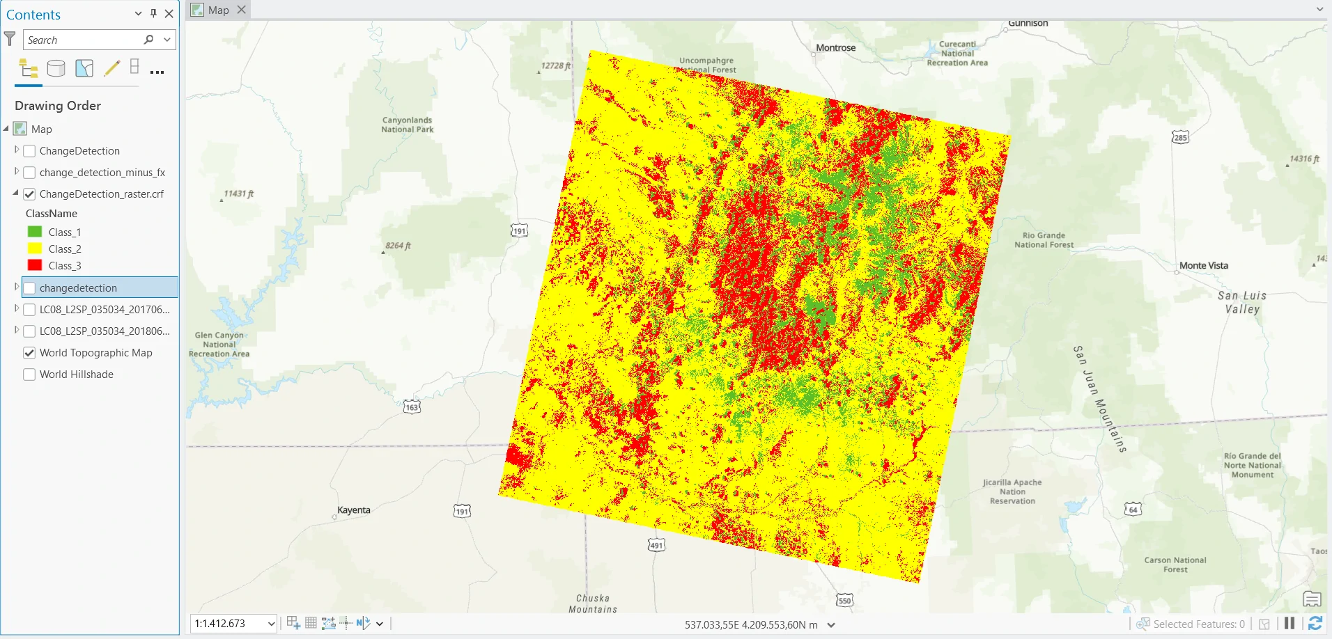
The result will be shown at the image below.

Last, we can convert raster data above into features format (table data), so we can analyze more the result of change detection into other analyze (i.e. summary area, statistic value).

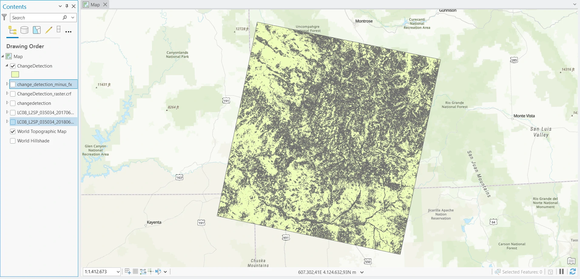
Raster Calculator

In this part, we use a process to calculate difference value in raster. By utilize Minus tools under Image Analyst Tools, we can subtracts the value of the two inputs raster on a cell-by-cell basis.

This tool just needed 2 inputs and output name and the result will be shown at the below.

Conclusion

The result of these 2 methods almost similiar (in some parts) because these methods have same basic process (i.e. applying image differencing, subtracting corresponding pixel values at each pixel). The advance methods for change detection can we read and discuss more at this page.