Finding the Shortest Path: A Simple Step-by-Step Guide

geospatial

map

Optimization

Introduction

Navigating a city efficiently—whether on foot, by bike, or by car—often comes down to finding the shortest and most optimal route. Using graph-based mapping techniques, we can calculate the best path between two locations based on real-world road networks. Here’s how the process works in three simple steps:

• Download and Create a Graph of the Area 🗺️
• Find the Nearest Nodes to Start and End Points 📍
• Compute the Shortest Path 🏁

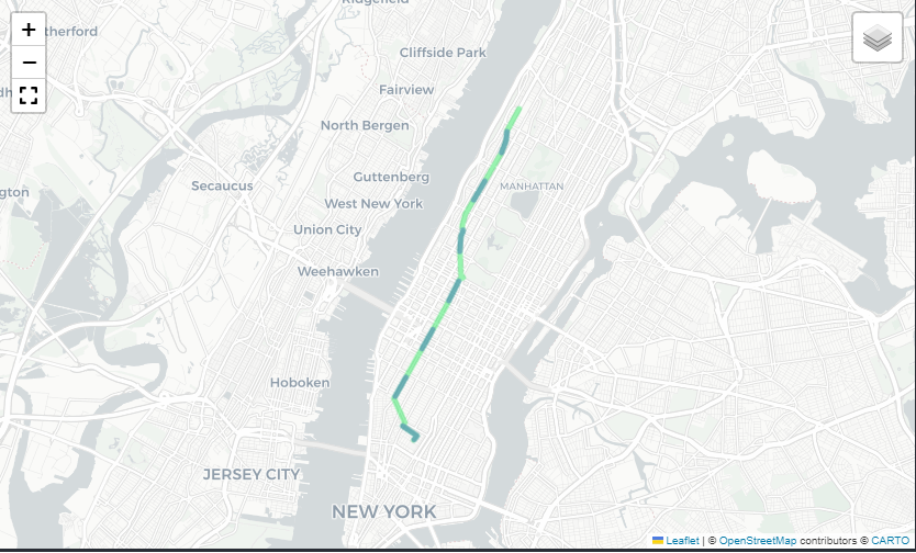
The result? A clear, optimized path from origin to destination, ready to be visualized on a map or used for navigation. 🚀

The Code

By calling maps.shortest_path, we can do all steps above, from retrive graph of specific area, find the Nearest Nodes to Start and End Points, and generate shortest path.

path, graph = maps.shortest_path(location='Manhattan, New York, USA', 
                            origin_coords=[40.7295, -73.9965], 
                            destination_coords=[40.8075,-73.9626], network_type='drive', method='dijkstra')

This function requires the following parameters:

• location (string): location name
• origin_coords (list): coordinate of origin point
• destination_coords (list): coordinate of destination point
• network_type (string): What type of street network to retrieve [“all”, “all_public”, “bike”, “drive”, “drive_service”, “walk”]
• method (string): The algorithm to use to compute the path. [“dijkstra”, “bellman-ford”]

The result

This process powers everything from GPS navigation apps to smart city planning, helping users move around more efficiently while making data-driven decisions about urban mobility.