Complete Spatial Randomness
geospatial
map
Pattern
Introduction
Beyond questions of centrality and extent, spatial statistics on point patterns are often concerned with how even a distribution of points is. By this, we mean whether points tend to all cluster near one another or disperse evenly throughout the problem area. Questions like this refer to the intensity or dispersion of the point pattern overall. This techniques all derive from Ripley (1988) and involve measurements of the distance between points in a point pattern.
Theory
Ripley’s alphabet of functions, focuses on the distributions of two quantities in a point pattern: nearest neighbor distances and what we will term “gaps” in the pattern. They derive from seminal work by Brian D Ripley, on how to characterize clustering or co-location in point patterns. Each of these characterizes an aspect of the point pattern as we increase the distance range from each point to calculate them.
Ripley’s G
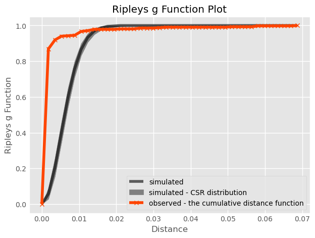
The first function, Ripley’s G, focuses on the distribution of nearest neighbor distances. That is, the function G summarizes the distances between each point in the pattern and its nearest neighbor. Ripley’s G keeps track of the proportion of points for which the nearest neighbor is within a given distance threshold, and plots that cumulative percentage against the increasing distance radii. The distribution of these cumulative percentages has a distinctive shape under completely spatially random processes.
The intuition behind Ripley’s G goes as follows: we can learn about how similar our pattern is to a spatially random one by computing the cumulative distribution of nearest neighbor distances over increasing distance thresholds, and comparing it to that of a set of simulated patterns that follow a known spatially random process. Usually, a spatial Poisson point process is used as such reference distribution.
Thinking about these distributions of distances, a “clustered” pattern must have more points near one another than a pattern that is “dispersed”; and a completely random pattern should have something in between. Therefore, if the G function increases rapidly with distance, we probably have a clustered pattern. If it increases slowly with distance, we have a dispersed pattern. Something in the middle will be difficult to distinguish from pure chance.
Ripley’s F
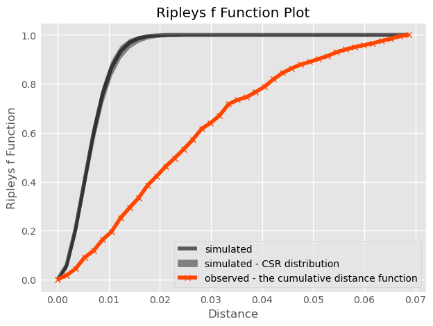
The second function we introduce is Ripley’s F. Where the G function works by analyzing the distance between points in the pattern, the F function works by analyzing the distance to points in the pattern from locations in empty space. That is why the F function is called the the empty space function, since it characterizes the typical distance from arbitrary points in empty space to the point pattern.
If the pattern has large gaps or empty areas, the F function will increase slowly. But, if the pattern is highly dispersed, then the F function will increase rapidly. The shape of this cumulative distribution is then compared to those constructed by calculating the same cumulative distribution between the random pattern and an additional, random one generated in each simulation step.
Dataset
Load dataset
In this project we will reused previous dataset from Point Pattern Analysis. To make things more clear, we’ll use the Flickr photos for the most prolific user in the dataset (ID: 95795770) to show how different these results can be.
db = pd.read_csv(r"..\map\tokyo_clean.csv")
db = gpd.GeoDataFrame(db, crs="EPSG:4326",geometry=gpd.points_from_xy(db.longitude, db.latitude))
db = db.query('user_id == "95795770@N00"')
| user_id | longitude | latitude | date_taken | photo/video_page_url | x | y | geometry | |
|---|---|---|---|---|---|---|---|---|
| 46 | 95795770@N00 | 139.733 | 35.6375 | 2010-01-09 12:31:00.0 | http://www.flickr.com/photos/95795770@N00/4257779201/ | 1.55551e+07 | 4.25085e+06 | POINT (139.73344 35.637486) |
| 70 | 95795770@N00 | 139.718 | 35.6387 | 2007-06-15 14:02:36.0 | http://www.flickr.com/photos/95795770@N00/551033440/ | 1.55534e+07 | 4.25102e+06 | POINT (139.718166 35.638666) |
| 84 | 95795770@N00 | 139.734 | 35.6443 | 2012-07-22 14:51:20.0 | http://www.flickr.com/photos/95795770@N00/7620079764/ | 1.55551e+07 | 4.25179e+06 | POINT (139.733917 35.644336) |
| 92 | 95795770@N00 | 139.734 | 35.6375 | 2006-10-19 06:34:58.0 | http://www.flickr.com/photos/95795770@N00/273401558/ | 1.55551e+07 | 4.25086e+06 | POINT (139.73355800000002 35.637532) |
| 114 | 95795770@N00 | 139.741 | 35.6621 | 2007-09-16 07:52:15.0 | http://www.flickr.com/photos/95795770@N00/1389657314/ | 1.55559e+07 | 4.25423e+06 | POINT (139.7409 35.66211) |
The Code
By calling maps.spatial_randomness, we can calculate spatial randomness Ripley with 3 types of Ripley - G, K, F. This function will return plot and dataframe that contain distance, observed, simulated, pvalue.
result = maps.spatial_randomness(main_data, col_list= ['longitude','latitude'], support=100, types='g')
This function requires the following parameters:
- main_data (
geodataframe): Data location and value - types (
string): type of Ripley’s. namlyg, k, f - col_list (
list): list of columns name to get coordinat in main data - support (
list): the exact distance values used to evalute the statistic
The result
Result The Table
| distance | observed | simulated | pvalue | |
|---|---|---|---|---|
| 0 | 0 | 0 | 0 | 0 |
| 1 | 0.0176018 | 0.0176018 | 0.057 | 0 |
| 2 | 0.0440044 | 0.0440044 | 0.207 | 0 |
| 3 | 0.090209 | 0.090209 | 0.404 | 0 |
| 4 | 0.117712 | 0.117712 | 0.599 | 0 |
Ripley’s G
On the left, we plot the G(d) function, with distance-to-point (d) on the horizontal axis and the fraction of nearest neighbor distances smaller than d on the right axis. The empirical cumulative distribution of nearest neighbor distances is shown in red. Black line represents the average of all simulations, and the darker gray band around it represents the middle 95% of simulations (like the random pattern shown in the previous section) are shown.
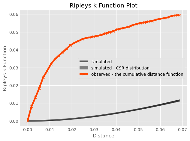
Ripley’s K
Ripley’s F