Topological Measures of Geographical Surfaces
geospatial
map
topological
Isolation and Prominence of country populations 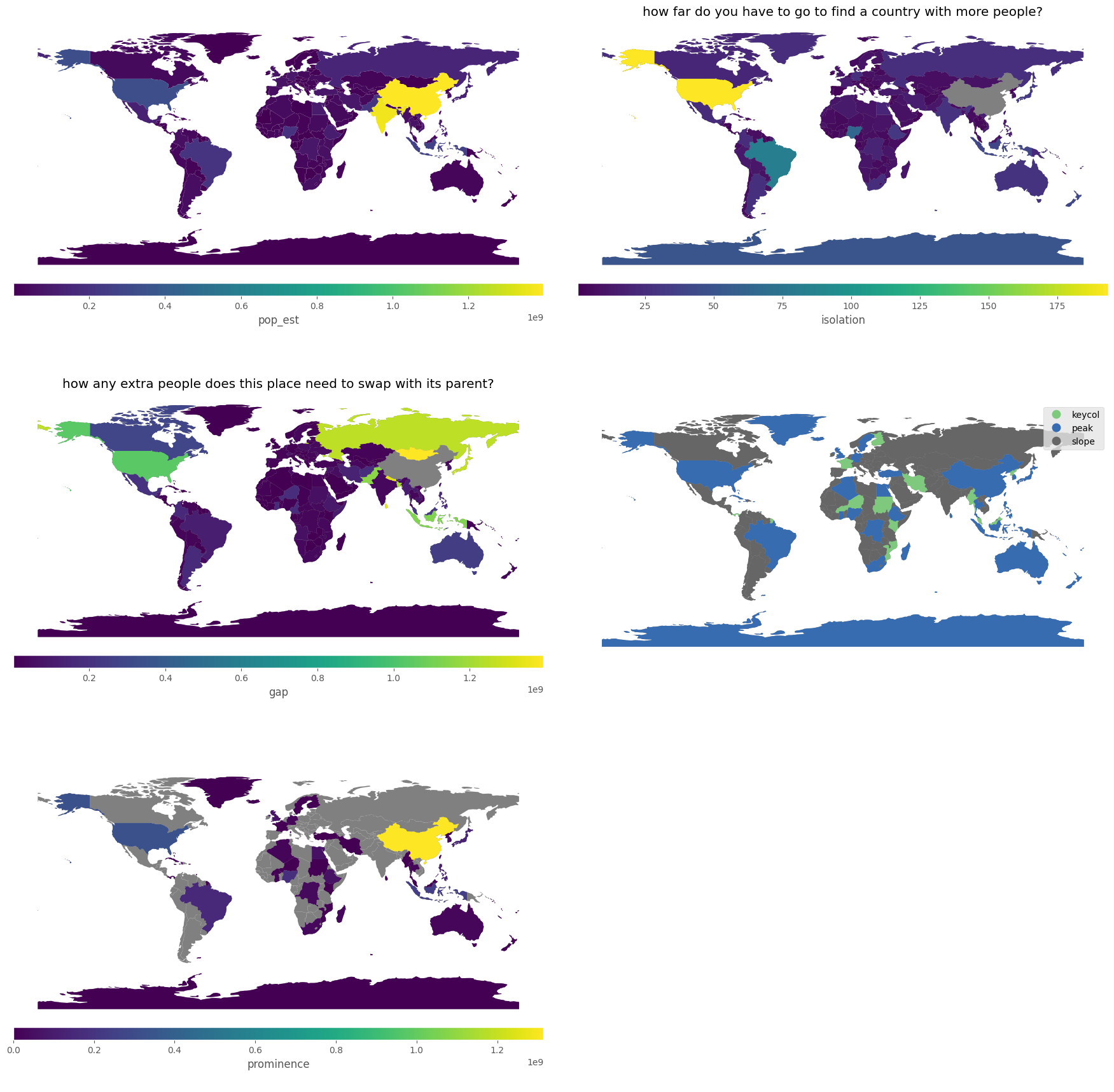
Introduction
Topographical measures focus on the shape of a surface. In physical geography, prominence and isolation are both topographical measures that refer to how high (or how `dominant`) a mountain is relative to its landscape. Mathematically, if we represent `elevation` with a surface (like a Digital Elevation Model, or DEM), then this becomes a way to characterize the local maxima, minima, and/or saddle points of a given surface.
Theory
Prominence (and isolation) are intricately connected to the local extrema and concavity/convexity of a surface, and provide useful ways to think about the structure of a geographical distribution.
In a physical sense, the isolation of a mountain peak is the distance you have to travel to find a higher point on the surface. So, the common example given, say, on Wikipedia, is that Mount Everest has an “infinite” isolation, since it is the highest point on Earth’s surface. The nearby peak K2, the second-highest mountain on Earth is relatively close to Everest, so K2 has quite a low isolation. However, Aconcauga, the tallest peak in the Western Hemisphere, is about 1,000 meters shorter than K2, but way more isolated, since the distance from it to the nearest highest point is very large. So, isolation is a measure of horizontal distance.
In contrast, prominence is a measure of vertical distance, describing the gap between the peak’s elevation and the “highest” low point between it and its parent peak. We use prominence because it tells you how high a peak/local maxima is relative to its surroundings.
Things are complicated somewhat when we’re dealing with irregular or dis-continuous relief. When dealing with mountains and elevation, we know that elevation is a surface that changes (relatively) smoothly. In contrast, most of our vector data does not change smoothly. Despite this, we can still use these notions of isolation and prominence to measure the relative contrasts between parts of a geographcial surface.
Dataset
Load dataset
we used population of countries dataset. we called the natural earth dataset from geopandas We’ll use the population estmate (pop_est) as a kind of elevation.
natearth = gpd.read_file(gpd.datasets.get_path('naturalearth_lowres'))
| pop_est | continent | name | iso_a3 | gdp_md_est | geometry | |
|---|---|---|---|---|---|---|
| 0 | 889953 | Oceania | Fiji | FJI | 5496 | MULTIPOLYGON (((180 -16.067132663642447, 180 -16.555216566639196, ))) |
| 1 | 5.80055e+07 | Africa | Tanzania | TZA | 63177 | POLYGON ((33.90371119710453 -0.9500000000000001, 34.07261999999997 -1.0598199999999451,)) |
| 2 | 603253 | Africa | W. Sahara | ESH | 907 | POLYGON ((-8.665589565454809 27.656425889592356, -8.665124477564191 27.589479071558227, )) |
| 3 | 3.75893e+07 | North America | Canada | CAN | 1736425 | MULTIPOLYGON (((-122.84000000000003 49.000000000000114, -122.97421000000001 49.00253777777778, ))) |
The Code
By calling maps.topo_analysis_map, we can generate 5-6 map plot that will give some insights about topological from our data.
result = maps.topo_analysis_map(main_data, col_list='pop_est')
This function requires the following parameters:
- main_data (
geodataframe): Data location and value - col_list (
list): targeted column
The result
At the 1st sub-image, explain about how perfect dataset to think about isolation/prominence, since we have big gaps between the highest population points in each continent.
At the 2nd and 3rd sub-image, we can see that the isolation for China is infinite, since there is no country with a larger population. However, the isolation for India is only the distance from China to India (27). The isolation for the US, however, is much larger, and reflects the distance from the US to India (which just happens to be closer than China). The fourth-most populous country, Indonesia, is closer to China than India, its isolation is the distance from Indonesia to China. Last, you see Brazil, 5th most populous country, has US as a parent, with an isolation distance of 82.
At the 4th and 5 th sub-image, you can see that the first key col country, France, is included around the 25-country mark, wheras before that most included countries are peaks, disconnected from one another. You can see the full map of classifications, alongside the prominence of each country.