Change Predition at Spatial and Temporal
geospatial
map
model
optimization
Have we ever looked out at a forest or a stretch of farmland and wondered, “What will this land look like in 10 years?” It’s a fascinating question—one that becomes increasingly urgent in the face of urban expansion, climate change, and evolving agricultural practices.
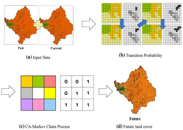
In this project, we explored how machine learning and spatial models can help us uncover patterns and predict future land use changes. At the heart of this work lies a powerful modeling framework: CA-Markov, a hybrid technique that blends the statistical insights of Markov chains with the spatial awareness of Cellular Automata.
Theory - What is a CA-Markov Model?
To understand CA-Markov, let’s break it down into two core components:
Markov Chains: Learning from the Past
Markov models look at how land categories—like forest, farmland, urban areas—have changed over time. By analyzing historical satellite imagery or land classification data, the model estimates the likelihood of transitions. For example, if data shows that 20% of a forested area consistently converts to farmland every decade, the model uses that probability to simulate future transitions. Think of it as using history as a guidebook for what might happen next.
Cellular Automata: The Power of Neighborhood Influence
Here’s where things get spatial. Cellular Automata (CA) models divide land into a grid of cells. Each cell’s future state doesn’t just depend on its own history—it also depends on the behavior of its neighbors. If surrounding land is turning into urban sprawl, the pressure for a single cell to urbanize increases.This mirrors how land change works in the real world: it’s rarely isolated. Urban growth, agricultural expansion, or deforestation tend to ripple out from existing areas.
Why Use CA-Markov for Land Use Prediction?
The real Interest happens when we combine these two techniques. While Markov Chains bring the temporal dynamics (how things change over time), Cellular Automata add the spatial context (where things change and why). Together, the CA-Markov model allows us to create more grounded, realistic simulations of future land use.
This approach is especially useful for:
- Environmental planning – Predicting deforestation or urban encroachment
- Agricultural development – Understanding how farmlands might expand or shrink
- Policy modeling – Assessing the long-term impact of land management decisions
Models like CA-Markov don’t just sit in academic papers. They can be embedded in dashboards, used in conservation projects, or integrated with GIS platforms to help planners and communities visualize the future—and make smarter decisions today.
How We Built the Model
To bring this model to life, we need:
- Collected historical land use maps via satellite imagery
- Pre-processed the data to align spatial layers and classification systems
- Used transition matrices from Markov analysis to understand probabilities
- Integrated the spatial patterns using CA rules
- Simulated multiple future scenarios under different assumptions (e.g., no intervention vs. conservation policies)
Dataset
For this project, we present a case study for Colombia, focusing on the Department of Caquetá in the southwestern region. We have land use data from five time periods: 2000–2002, 2005–2009, 2010–2012, 2018, and 2020, and our goal is to predict the land use changes expected by 2030. This data was provided by the Instituto de Hidrología, Meteorología y Estudios Ambientales (IDEAM) and processed as raster files with integer values representing each land use category.
Load dataset
We will use the processed rasters data in the following order:
- Download the land use from the national authorities for the 5 periods of evaluation.
- Clip for the region of interest (Department of Caquetá)
- Transform shapefile into raster with a 250 meter resolution and keeping values as integer values
- Keep the same extent after resample it into 250 meters.
data_path = "../CA-Markov_Rasters_Caqueta/"
valid_classes = [11, 12, 13, 21, 22, 23, 24, 31, 32, 33, 41, 42, 51, 52]
cloud_value = 99
raster_files = ['2000_2002.tif', '2005_2009.tif', '2010_2012.tif', '2018.tif', '2020.tif']
raster_titles = ['2000_2002', '2005_2009', '2010_2012', '2018', '2020']

#Load rasters
raw_rasters = {}
for file in raster_files:
    with rasterio.open(os.path.join(data_path, file)) as src:
        raw_rasters[file] = src.read(1).astype(float)
Pre-Processing
First we need to pre-processing our raster data to get more precise and accurate data. This process separate into 3 steps:
- Cleansing - to clean our rasters from outliers values if exist, the following code cleans each map by checking every pixel – if a pixel’s value isn’t one of our 14 valid land use codes, it gets replaced with a missing value (NaN).
- Filling data - Next, it fills in any gaps by borrowing values from the most recent map available, so there aren’t any empty spots.
- Clipping - Finally, it uses a 2020 map as a guide to clip all the maps to just the area we’re interested in, so any pixel outside that area is set to NaN.
By calling maps.clip_outlier_raster, maps.filler_raster and maps.clip_raster, we can perform pre-processing to cleansing, filling, and clipping data to all our raster data. each function has default parameter for difference condition.
cleaned_rasters = [maps.clip_outlier_raster(raw_rasters[file], valid_classes) for file in raster_files]
filled_rasters = maps.filler_raster(cleaned_rasters, types='last')
raster_cleaned = maps.clip_raster(filled_rasters, raster_files, data_path+'/2020.tif', classes=valid_classes)
This function requires the following parameters:
- main_raster (
raster or list of raster): raster data - classes (
list): list of raster band - types (
string): type of filling process - list_raster_name (
list): list of raster name - reference_raster_path (
string): path of raster as a reference
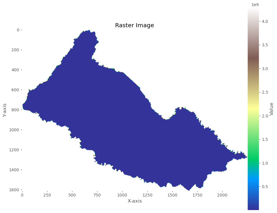
The output of this process can be seen below.
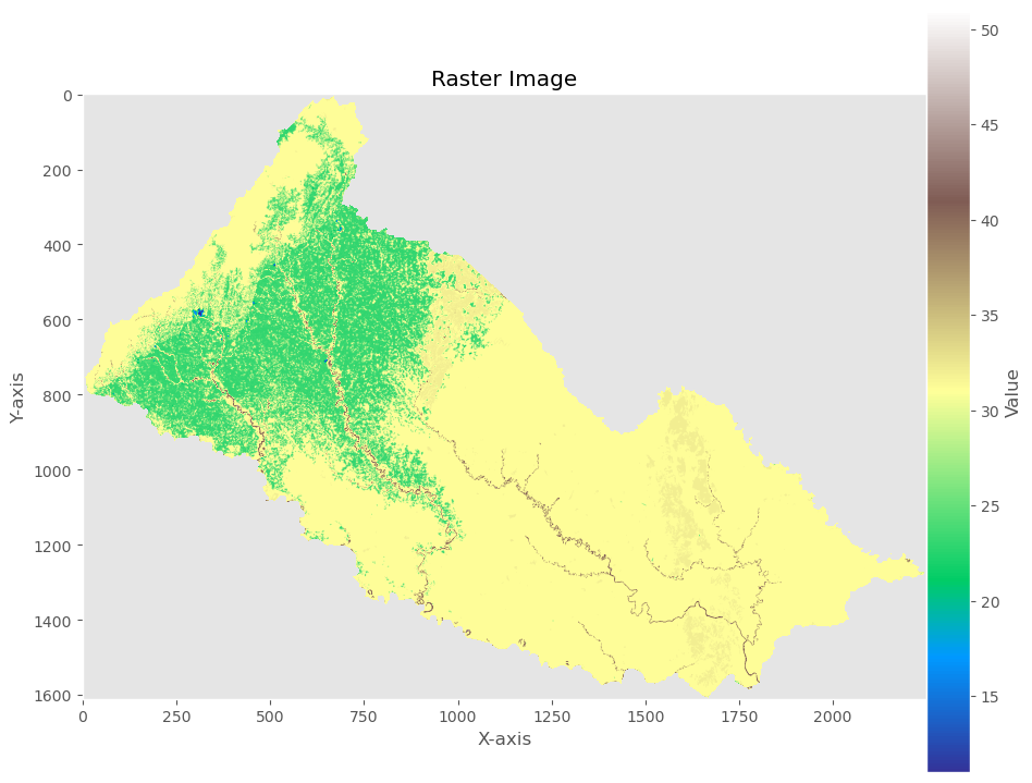
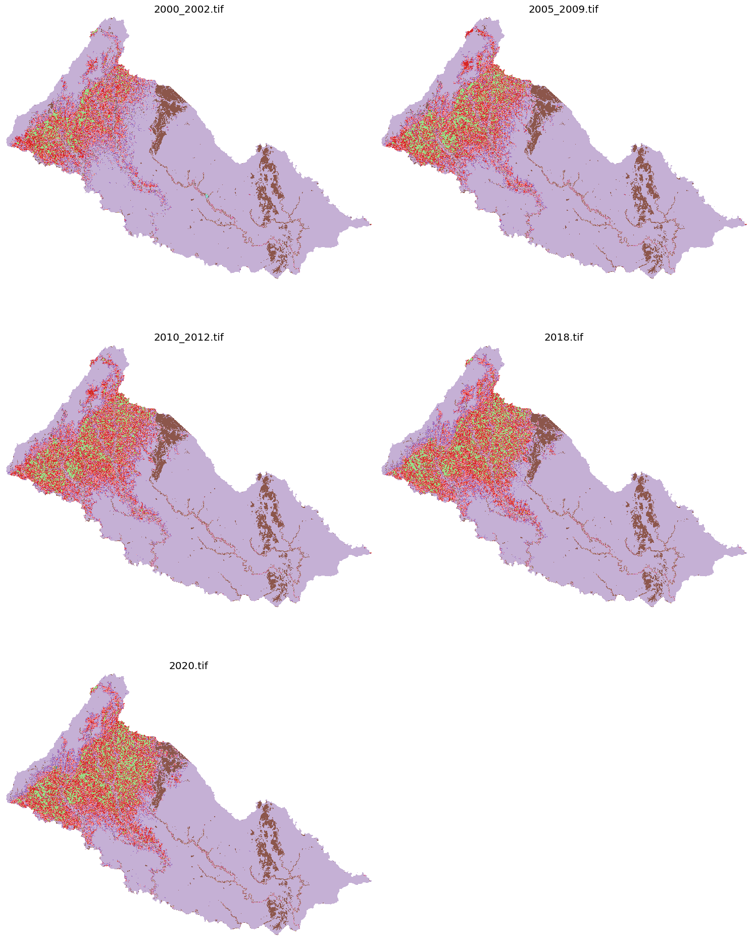
additionally, we can combine the name and the array of raster into single variable to make easier to iterate and create temporal prediction (i.e. the image below that showing all our raster into single image). We can combine all of them into single dictionary with their name as a key.
#Convert to dictionary with integer values, keeping the same names
rasters = {file: raster.astype(int) for file, raster in zip(raster_files, filled_rasters)}

plt.figure(figsize=(15, 20))
for i, (name, raster) in enumerate(raster_cleaned.items(), 1):
    plt.subplot(3, 2, i)
    plt.imshow(raster, cmap='tab20', vmin=11, vmax=52)
    plt.title(name)
    plt.axis('off')
plt.tight_layout()
plt.show()
Modeling
Now let´s take two rasters to build our transition probability. This process help us to calculate and determine how likely the raster change in train data duration. First, we will examine transition in our raster to give us more information how this land change. For this project, we can use 2018 and 2020 raster data, and hopefully it might be enough to predict next year (e.i. at 2030). To create transition matrix, we can use this function map.transition_matrix_raster to give us transition change between each band.
transition_probs, transition_counts, transition_percent = maps.transition_matrix_raster(rasters['2018.tif'], rasters['2020.tif'], valid_classes)
This function requires the following parameters:
- from_raster (
raster or list of raster): the old raster data - to_raster (
raster): the new raster data - classes (
list): list of raster band - non_zero (
boolean): add small number to avoiding zero value in our data
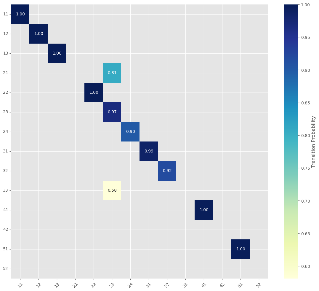
To visualizing the result, we can use heatmap function like follow visual.heatmap_exist(transition_probs, classes, limit=0.2 , title=None, labels=['','']) and the plot can be shown below that give us an information about Transition Probability Matrix (2018-2020).
This function requires the following parameters:
- transition_probs (
array): array value - limit (
float): the limit of non-correlation / non-transition data
In the following process we will recreate transition probability but from train data (2010 to 2018) and use test data (2020) raster to evaluate our model:
- Grab Training Maps: - By load two maps, one from the beginning of a training period (e.g., 2010–2012) and one from the end of that period (e.g., 2018).
- Build the Transition Matrix - It then compares these two maps to see how many pixels changed from one land-use type to another. This gives us a transition matrix showing, for example, how many “Forest” pixels turned into “Urban” pixels.
- Regularize and Calculate Probabilities - To avoid division errors (like dividing by zero), a tiny number (epsilon) is added, and the counts are converted into probabilities. This tells us the chance of each land-use change happening.
- Determine the Time Gap - The script figures out how many years lie between the end of the training period (2018) and the test year (2020).
- Predict the Future Map - By raising the transition matrix to the power corresponding to the number of years in that gap, it predicts what the land-use map should look like in 2020. Essentially, it uses the training data to forecast the changes over time.
- Compare Prediction with Reality - It loads the actual 2020 map and compares it with the predicted map, focusing only on the valid land-use types.
- Measure Performance - Evaluate the model
To do those steps, we can utilize this function maps.temporal_validation_raster. In general, this function will need raster data, selected train data, test data, and time label. This function requires the following parameters:
- raster_files (
raster or list of raster): the raster data - train_data (
list): list of raster name as train - test_data (
list): list of raster name as test - time_label (
list): list of label from training and testing - classes (
list): list of raster band - year_pairs (
list): list of year pair name
accuracy, kappa, predicted = maps.temporal_validation_raster(raster_files, train_data=[rasters['2010_2012.tif'],rasters['2018.tif']],
                                            test_data=rasters['2020.tif'], time_label=[2010,2018,2020], classes=valid_classes,
                                            year_pairs = [(2000, 2002), (2005, 2009), (2010, 2012), (2018, 2018), (2020, 2020)], )
This is an output from above process. As shown below:
Validation Report (2010-2018 → 2020):
- Time steps: 2 years
- Valid pixels: 1483312 (40.9% of total)
- Accuracy: 93.74%
- Cohen's Kappa: 0.872
- We determine time steps for 2 years due to our data has the smallest time steps in 2 years.
- the valid pixels in this process is around 1.483.312 pixels
- for evaluation, we got:
- Accuracy is around 93.74%
- Cohen’s Kappa: 0.872
Theory - What Is Cohen’s Kappa?
Cohen’s Kappa is used for measuring the agreement between two evaluators. The kappa score measures the degree of agreement between the true values and the predicted values also known as inter-rater reliability.
What is Inter-Rater Reliability?
Imagine two teachers are grading the same set of student essays. We want to know how much they agree on the grades. That’s inter-rater reliability — it tells us how consistently two (or more) people are making the same judgments. So if both teachers always give the same grade to each essay, the inter-rater reliability is high. If they often disagree, it’s low. But Wait — What If They Agree Just by Chance? Let’s say there are only two grades: “Pass” or “Fail”. If two teachers randomly guess “Pass” or “Fail” for each essay, they might still agree some of the time — just by luck. So we need something smarter than just counting how often they agree.
That’s Where Cohen’s Kappa Comes In. Cohen’s Kappa is a way to measure inter-rater reliability while taking into account agreement by chance. It answers: “How much better is their agreement than random guessing?”
The Kappa statistic varies from 0 to 1, where: 0 = agreement equivalent to chance 0.1 – 0.20 = slight agreement 0.21 – 0.40 = fair agreement 0.41 – 0.60 = moderate agreement 0.61 – 0.80 = substantial agreement 0.81 – 0.99 = near perfect agreement 1 = perfect agreement
That is it, our calculation and data has great accuracy and and cohen kappa value. To get more details about our calculation, we can examine a long report of scoring process below.
classification_report
              precision    recall  f1-score   support

          11       0.95      0.81      0.87       688
          12       0.78      1.00      0.87        87
          13       0.00      0.00      0.00         0
          21       0.00      0.00      0.00         0
          22       0.00      0.00      0.00         0
          23       0.95      0.79      0.86    307422
          24       0.00      0.00      0.00         0
          31       1.00      0.99      0.99   1020586
          32       0.98      0.89      0.94    140449
          33       0.00      0.00      0.00         0
          41       0.00      0.00      0.00         0
          51       0.99      1.00      0.99     14080

    accuracy                           0.94   1483312
   macro avg       0.47      0.46      0.46   1483312
weighted avg       0.99      0.94      0.96   1483312


accuracy_score =  0.9374
balanced_accuracy_score =  0.9131
precision score =  0.9866
recall score =  0.9374

F1 score =  0.9604
F_beta score =  0.9757
AUC of ROC for ovo = 0.9553
Plot Confusion Matrix
Confusion Matrix in Table Format
| 11 | 12 | 13 | 21 | 22 | 23 | 24 | 31 | 32 | 33 | 41 | 42 | 51 | 52 | classes_From-To | |
|---|---|---|---|---|---|---|---|---|---|---|---|---|---|---|---|
| 0 | 100 | 0 | 0 | 0 | 0 | 0 | 0 | 0 | 0 | 0 | 0 | 0 | 0 | 0 | 11 |
| 1 | 0 | 100 | 0 | 0 | 0 | 0 | 0 | 0 | 0 | 0 | 0 | 0 | 0 | 0 | 12 |
| 2 | 0 | 0 | 100 | 0 | 0 | 0 | 0 | 0 | 0 | 0 | 0 | 0 | 0 | 0 | 13 |
| 3 | 0 | 0 | 0 | 19.44 | 0 | 80.56 | 0 | 0 | 0 | 0 | 0 | 0 | 0 | 0 | 21 |
| 4 | 0 | 0 | 0 | 0 | 100 | 0 | 0 | 0 | 0 | 0 | 0 | 0 | 0 | 0 | 22 |
| 5 | 0.01 | 0.01 | 0 | 0.07 | 0 | 96.68 | 2.91 | 0 | 0.09 | 0.19 | 0.04 | 0 | 0 | 0 | 23 |
| 6 | 0.01 | 0.01 | 0 | 0.02 | 0 | 8.93 | 90 | 0.12 | 0.76 | 0.14 | 0 | 0 | 0 | 0 | 24 |
| 7 | 0 | 0 | 0 | 0.01 | 0 | 0.67 | 0.57 | 98.57 | 0.16 | 0.02 | 0 | 0 | 0 | 0 | 31 |
| 8 | 0 | 0 | 0 | 0.01 | 0 | 3.15 | 4 | 0.25 | 91.91 | 0.67 | 0 | 0 | 0 | 0 | 32 |
| 9 | 0 | 0 | 0 | 0.17 | 0 | 58.1 | 6.12 | 0.08 | 15.64 | 16.78 | 0 | 0 | 3.11 | 0 | 33 |
| 10 | 0 | 0 | 0 | 0 | 0 | 0.22 | 0 | 0 | 0 | 0.07 | 99.71 | 0 | 0 | 0 | 41 |
| 11 | 0 | 0 | 0 | 0 | 0 | 0 | 0 | 0 | 0 | 0 | 0 | 0 | 0 | 0 | 42 |
| 12 | 0 | 0 | 0 | 0 | 0 | 0.08 | 0.02 | 0.01 | 0.01 | 0.05 | 0 | 0 | 99.83 | 0 | 51 |
| 13 | 0 | 0 | 0 | 0 | 0 | 0 | 0 | 0 | 0 | 0 | 0 | 0 | 0 | 0 | 52 |
Prediction
Now, let’s apply the CA-Markov model using the prediction matrix we built, which allowed us to calculate the 2020 land use with high accuracy. This approach might also be effective for predicting future land use. To do that, we utilize model_pred.ca_markov_model to create prediction for 2030.
This function requires the following parameters:
- current_state (
raster or list of raster): current or latest raster to predict next state. - transition_matrix (
array): transition matrix from previous process using train data - classes (
list): list of raster band - steps (
int): step value that required to detemine at what time we we want to predict. (i.e. for create prediction for 2030, we need steps=5 to get 2020 or latest data to 2030 with 5 steps and 2 years for step in our training)
predicted_2030_ = model_pred.ca_markov_model(
    current_state=rasters['2020.tif'],
    transition_matrix=transition_probs,
    classes=np.array(valid_classes),
    steps=5
)
The result
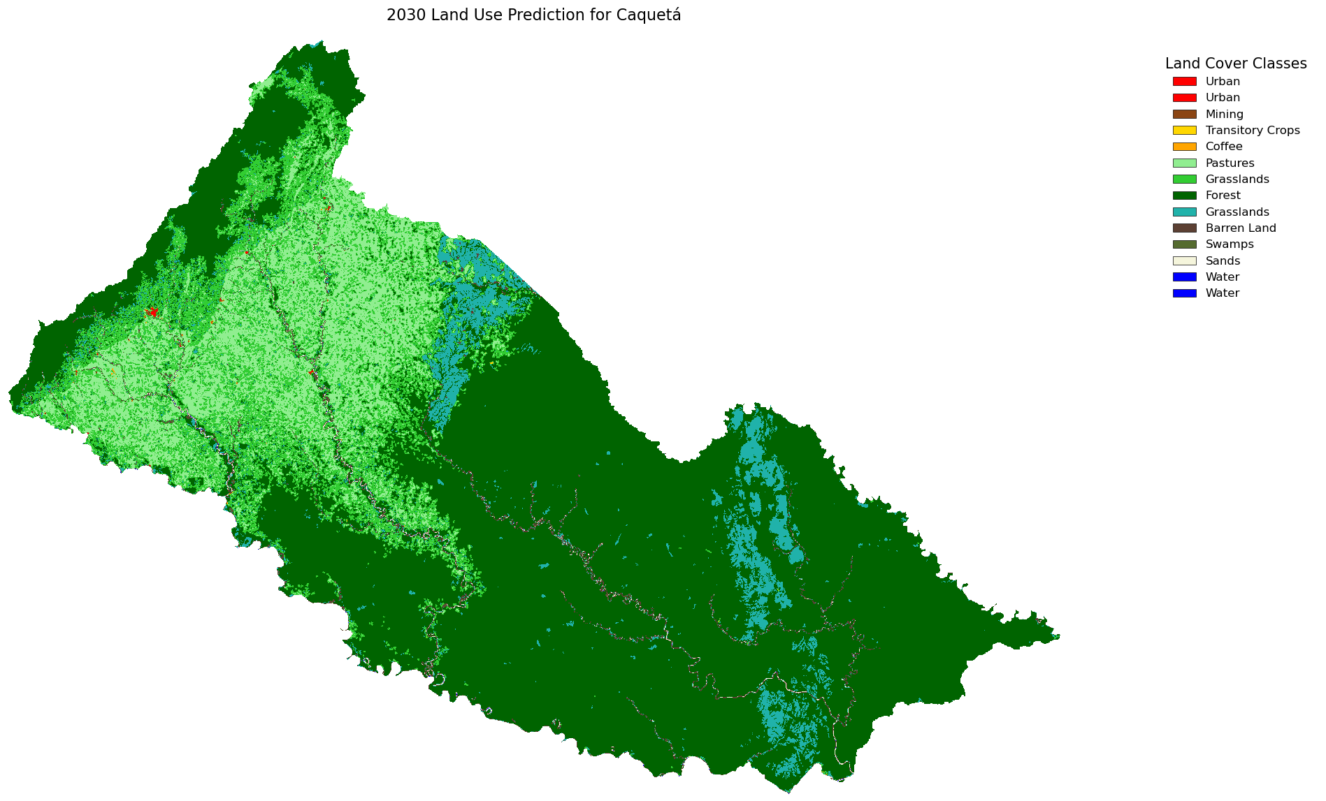
Now it’s time to plot our projection for 2030. But first, we’ll clip it with a mask to avoid not logical estimations around the borders. We can use this function maps.ca_markov_prediction to plot and clip our data and analize land cover that product by our model. We can add some label and legend into our result to give more information.
maps.ca_markov_prediction(train_data_path, classes, prediction, title='', figsize=(18, 12), color_dict=[], legend_labels=[])

masked_prediction = maps.ca_markov_prediction(data_path+'/2020.tif',classes=valid_classes, prediction=predicted_2030,
                                                title='2030 Land Use Prediction for Caquetá', figsize=(18, 12), color_dict=color_dict, legend_labels=legend_labels)
This function requires the following parameters:
- train_data_path (
string): location of raster file - classes (
list): list of raster band - prediction (
array): prediction result - title (
string): title of plot - figsize (
tuple): size of plot - color_dict (
dict): custom color mapping based on your specifications - legend_labels (
dict): custom legend labels - pred_name (string): prediction name file
To see more clearly how to data change and how our prediction result, we can create animation to comparing each raster or year and add prediction at the end of that animation as seen at image below.
Or we can generate table to see how Ha per pixel and percentage change from first raster (2000-2002) to the latest raster (2020) and with our rediction result. we utilize maps.comparing_raster to generate table to compare each raster.
# PARAMETERS
pixel_size = 250  # meters
ha_per_pixel = (pixel_size ** 2) / 10000  # 250x250 m => 6.25 ha per pixel

result = maps.comparing_raster(raster_data=[rasters['2000_2002.tif'],rasters['2005_2009.tif'],rasters['2010_2012.tif'],rasters['2018.tif'],rasters['2020.tif'],rasters['2030.tif']], labels=['2000_2002', '2005_2009','2010_2012','2018','2020','2030'], classes=valid_classes, ha_per_pixel=ha_per_pixel, legend_labels=legend_labels)
This function requires the following parameters:
- raster_data (
list): list of raster data in array type - labels (
list): label for each raster - classes (
list): list of raster band - ha_per_pixel (
int): ha per pixel - legend_labels (
dict): custom legend labels
| Land use | 2000_2002 | 2005_2009 | 2010_2012 | 2018 | 2020 | 2030 | % Change |
|---|---|---|---|---|---|---|---|
| Barren Land | 606.25 | 11287.5 | 4118.75 | 30131.2 | 15687.5 | 6125 | -60.9562 |
| Coffee | 0 | 0 | 0 | 550 | 550 | 550 | 0 |
| Forest | 7.07189e+06 | 6.79843e+06 | 6.65369e+06 | 6.37866e+06 | 6.28982e+06 | 6.28982e+06 | 0 |
| Grasslands | 1.17039e+06 | 1.12468e+06 | 1.12297e+06 | 1.21491e+06 | 1.24571e+06 | 1.24742e+06 | 0.13697 |
| Mining | 0 | 0 | 0 | 56.25 | 56.25 | 56.25 | 0 |
| Pastures | 950025 | 1.22919e+06 | 1.37618e+06 | 1.54543e+06 | 1.61444e+06 | 1.62391e+06 | 0.586502 |
| Sands | 0 | 0 | 0 | 0 | 0 | 0 | 0 |
| Swamps | 40993.8 | 19487.5 | 17687.5 | 8718.75 | 9262.5 | 9262.5 | 0 |
| Transitory Crops | 0 | 0 | 0 | 225 | 1931.25 | 318.75 | -83.4951 |
| Urban | 2212.5 | 3131.25 | 3193.75 | 4012.5 | 4368.75 | 1.33783e+07 | 306127 |
| Water | 34581.2 | 84493.8 | 92856.2 | 88000 | 88862.5 | 88862.5 | 0 |
Conclution
We looked at the CA-Markov projection from 2020 to 2030 and found that while most land uses like forest, water, and urban areas seem to stay stable, barren land and transitory crops are predicted to drop sharply, and grasslands and pastures show a slight increase.
This region is trending in deforestation due to the increase of grassland areas; urban areas should also increase, and barren areas should be more common unless there’s forest regeneration—which for this region might be difficult. We need to add restrictions to the CA-Markov model for categories like water or urban areas that are expected to grow, and I also think that using a two-year step might not fully reflect future reality.