Spatial interpolation

geospatial

map

interpolation

Estimating unknowns with spatial interpolation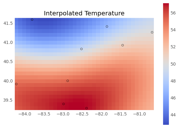

Introduction

Spatial interpolation is a process that uses known values from observations to estimate values at other unknown locations. This process is common in a number of scientific fields, such as meteorology and wildlife conservation. When it comes to meteorology, weather data is provided from a handful of weather stations in a given geography. From that information, meteorologists are asked to make predictions about what the weather will be at other locations.

There are many methods for performing spatial interpolation, including Inverse Distance Weighted (IDW) interpolation, Triangular Information Network (TIN) interpolation, and Kriging-based interpolation methods, to name a few. In this section, we’ll introduce to IDW interpolation as well as Ordinary Kriging (OK), which are two of the most common spatial interpolation methods that we’ll encounter.

Dataset

Load dataset

We’ll be interpolating the average daily temperature in Fahrenheit for the state of Ohio. The dataset we’ll leverage for this exercise was obtained from the National Oceanic and Atmospheric Administration’s (NOAA’s) National Centers for Environmental Information Climate Data Online portal at https://www.ncei.noaa.gov/cdo-web/datasets. We’ll be interpolating the temperatures for January 1, 2022.

path = r'..\map\book\C11'

main_data = path + f"\Ohio Temps.shp"
extend = path + f"\Ohio_State.shp"

Theory

Inverse Distance Weighted (IDW) interpolation

The IDW interpolation method uses sampled points to infer the value at an unknown location, whereby the effect of the sampled point on the prediction of the interpolated point diminishes as the distance between the sampled and interpolated point increases. This method adheres to Tobler’s First Law of Geography, which states everything is related, but near things are more related than distant things.

IDW limitation:

• the resulting interpolation’s accuracy can decrease if the distribution of the sampled points is unevenly distributed across the study area.
• the IDW method cannot produce interpolated values that are outside the minimum or maximum of the observed values.

Kriging-based interpolation

Kriging is a spatial interpolation method that leverages distance similarly to the IDW interpolation method but also leverages the degree of variation in sampled data points to interpolate unknown points. Kriging-based estimates are produced using a weighted linear combination of the sampled values around the unknown point. by using variography (empower with the spatial autocorrelation between the points measured using a fitted model to the observed points) the fitted model is thusly called a semivariogram. There are several variogram models that can be fit in most Kriging, applications including Gaussian, exponential, spherical, and linear. Kriging-based interpolation produces a surface of interpolated values that is much smoother than that of IDW. Using spatial interpolation, you can deduce the average temperature across the state and then include the interpolated values as an explanatory variable in some form of regression model to predict energy usage.

The Code

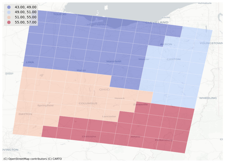
By calling maps.spatial_interpolation, we can weather stations reporting data for January 1, 2022 across Ohio, and calculate interpolation for area around them.

result = maps.spatial_interpolation(main_data, extend, col_name='TAVG',
                                    types='idw', search_radious= 3, power=2,
                                    variogram_model='gaussian',
                                    crs_meter=3347, crs_deg=4326, resolution = 25_000)

This function requires the following parameters:

• main_data (string): Data location and value
• shape (string): Shapefile location
• col_name (string): Targated column in main_data
• types (string): type of interpolation (scipy, IDW, krige)
• search_radious (int): a default value of 4, it determines how many nearest points will be used for idw calculation.
• power (int): a default value of 2, this is the power parameter from idw equation.
• variogram_model (string): Gaussian, exponential, spherical, and linear

The result

Nearest ND Interpolator

The Nearest ND Interpolator does a good job of picking up on the overall signal from the data, with temperatures decreasing as you move further north in the state.

IDW

The IDW interpolation does a good job of picking up on the overall signal from the data, with temperatures decreasing as you move further north in the state. It also picks up on the observation in the northeast of the state, which is a bit warmer than other locations in the surrounding area.

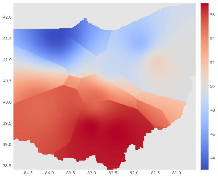
Kriging-based

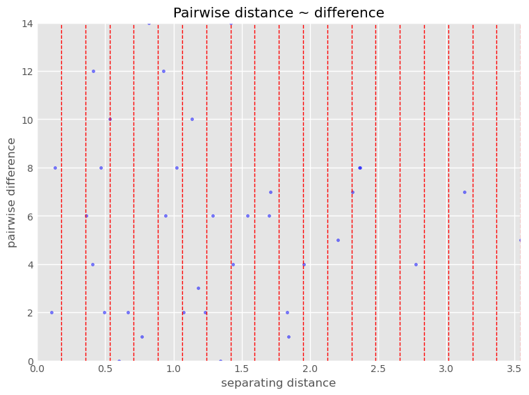
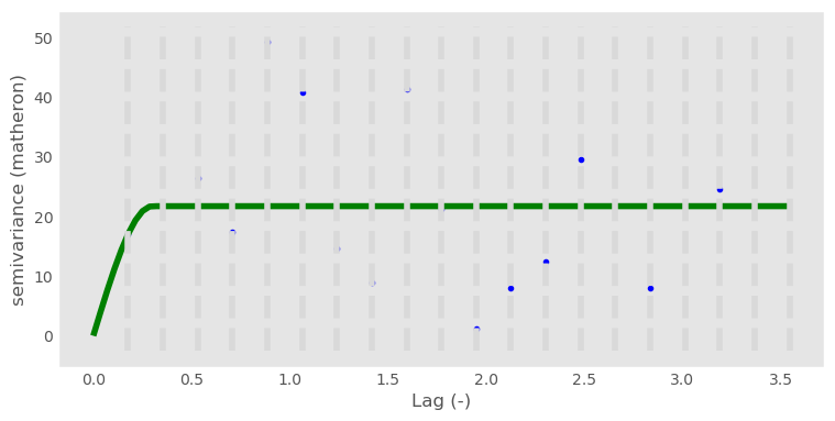
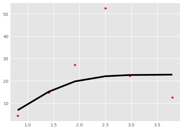
shows an empirical semivariogram using a Gaussian model. The Gaussian model does reasonably well fitting the points, even with the large outlier.

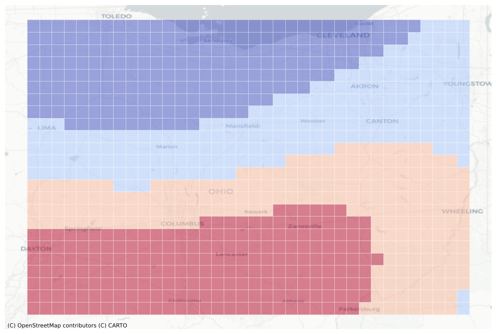
Compared to IDW, OK produces a surface of interpolated values that is much smoother than that of IDW. The values around the sampled observations are roughly the same as that of the IDW-based approach.