Developing Spatial Regression Models
geospatial
map
Pattern
Introduction
In this project, we will be discussing regression models and how they can be improved by incorporating spatial structures. Spatial structures can be an important facet of building into traditional regression models, but they are often overlooked. It is important to consider spatial structures and to build them into a regression model when the process that generated the source data is geographic in nature.
For example, Imagine that we operate a chain of high-end furniture stores and we’re trying to identify the best location for a future storefront that would maximize sales. Sales at our existing stores could be impacted by the number of cars that pass by the store every day, the proximity to other furniture stores, the number of new housing developments in nearby neighborhoods, and the affluence of the population in the vicinity.
Theory
A potential regression model could be used in one of two ways:
- To explain the relationship between a variable and store sales. The explanation is important because it allows you to model a phenomenon or relationship to understand it better and leverage this understanding to make more informed decisions in the future.
- To predict future store sales. Prediction can be very powerful, as it allows you to infer the future value at a particular location or future time based on information from historical data.
Simple Linear Regression Equation
The equation for simple linear regression is:
\[y = \beta_0 + \beta_1 \cdot x + \epsilon\]Where:
- ( \(y\) ) is the dependent variable (the variable we are trying to predict),
- ( \(\beta_0\) ) is the intercept of the regression line,
- ( \(\beta_1\) ) is the slope of the regression line (the change in ( \(y\) ) for a one-unit increase in ( \(x\) )),
- ( \(x\) ) is the independent variable (the predictor),
- ( \(\epsilon\) ) represents the error term (the difference between the observed and predicted values of ( \(y\) )).
Incorporating spatial fixed effects within the model
The incorporation of spatial proximity features was your first foray into teaching the model to think spatially. While these features benefited model performance and addressed the underlying premium visitors may be willing to pay to stay in close proximity to famous NYC attractions, they did not address all of the spatial structure present in the data.
As with neighborhoods across the country, underlying real estate values in NYC may vary from neighborhood to neighborhood. This underlying price structure in neighborhood real estate values could cause the host to pass along some or all of that cost to the potential renter of their Airbnb. This variation across space between the outcome variables and the explanatory, or predictor, variables is known as spatial nonstationarity.
One way to account for spatial nonstationarity is by adding spatial fixed effects. A fixed effect is a term commonly found in econometrics and is defined as an effect that is held constant within some cross-section of the data while other model parameters are allowed to vary.
Dataset
Load dataset
For this project, we are going to continue leveraging the New York City (NYC) Airbnb dataset that we’ve worked with in prior chapters. Our focus for this analysis will be attempting to build an explanatory model for nightly Airbnb rental prices.
We’ll subset the data to only include a handful of variables that may be indicative of nightly rental rates for Airbnbs in NYC. Here, you’ll select variables such as the neighborhood, the number of bedrooms and beds, the room type, and etc. With that subset process, we define a list of variables that will be used to explain the nightly Airbnb rental rate, there are ['accommodates', 'bedrooms','beds','review_scores_rating','rt_entire_home_apartment','rt_private_room','rt_shared_room'].
gdf = pd.read_csv(r'E:\gitlab\dataset\map\book\listings_manhattan_subset.csv')
gdf = gpd.GeoDataFrame(gdf)
| Unnamed: 0 | id | room_type | accommodates | bedrooms | beds | review_scores_rating | price | rt_entire_home_apartment | rt_private_room | rt_shared_room | log_price | |
|---|---|---|---|---|---|---|---|---|---|---|---|---|
| 0 | 0 | 2595 | Entire home/apt | 1 | 0 | 1 | 4.68 | 240 | 1 | 0 | 0 | 5.48064 |
| 1 | 2 | 6872 | Private room | 1 | 1 | 1 | 5 | 65 | 0 | 1 | 0 | 4.17439 |
| 2 | 3 | 6990 | Private room | 1 | 1 | 1 | 4.88 | 71 | 0 | 1 | 0 | 4.26268 |
| 3 | 11 | 12192 | Private room | 2 | 1 | 1 | 4.4 | 75 | 0 | 1 | 0 | 4.31749 |
| 4 | 15 | 15341 | Entire home/apt | 3 | 1 | 2 | 4.58 | 191 | 1 | 0 | 0 | 5.25227 |
The Code
By calling maps.spatial_regression, we can constructing an ordinary least squares (OLS) regression model and we will add more details in that model.
m_vars = ['accommodates', 'bedrooms','beds','review_scores_rating',
          'rt_entire_home_apartment','rt_private_room','rt_shared_room'
         ]

result, main_data_res = maps.spatial_regression(main_data, target='log_price', name_y='price', name_x=m_vars, fixed_effect= None)
This function requires the following parameters:
- main_data (
geodataframe): Data location and value - target (
string): targeted column (the outcome variables) - name_y (
string): name of y axis or the outcome variables - name_x (
list): list of dependent variables (the explanatory) - fixed_effect (
list): list of columns that has variation across space between the outcome variables and the explanatory
The result
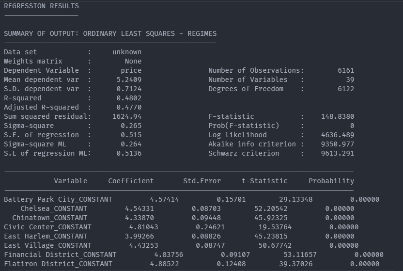
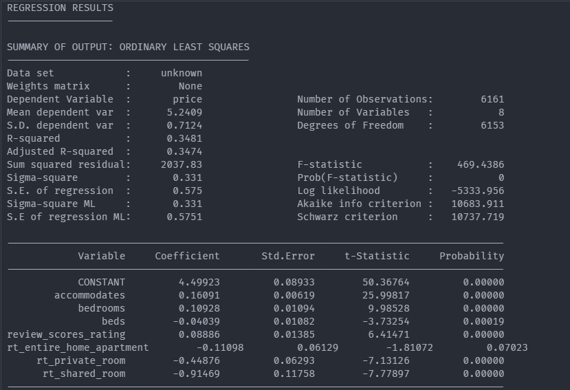
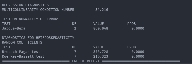
Result The Report without fixed_effect
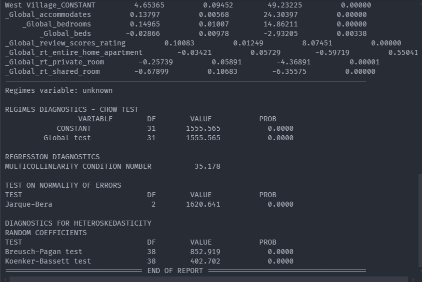
Result The Report with fixed_effect