Determining suitability

arcgispro

geospatial

map

esri

In this project, we will solve a common GIS problem: determining which areas are most suitable for a specific land-use purpose.

Raster 101

A raster is that it is composed of a grid of cells, instead of discrete x, y coordinates, that define geographic entities. The cells contain values that are used to record and define geographic phenomena on the surface of the earth. Each raster cell represents a portion of the earth, such as a square meter or square mile, and usually has an attribute value such as elevation, soil type, or vegetation class associated with it.

A surface, which is made up of raster cells, can be discrete data, which means that it shows distinct and discernible regions on a map, such as soil types, or it can be continuous data, which means that there are smooth transitions between variations in the range of data. Elevation data is one of the most common uses of a continuous raster. Typical raster datasets are extremely detailed and store a large amount of information, recording information about each cell.

Every raster cell has a value. Some cells may have a value of zero (for instance, representing no precipitation), and some cells may have a value of NoData, which means that no values were recorded for that cell. NoData cells are ignored in raster calculations.

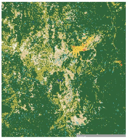
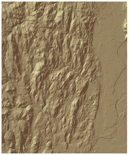
About images: (Left) This raster of discrete data represents land cover. Data courtesy of Lake Tahoe Data Clearinghouse, US Geological Survey. (Right) This raster of continuous data represents elevation. Data courtesy of the Oce of Geographic Information (MassGIS), and the Commonwealth of Massachusetts Information Technology Division.

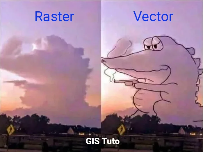
The simple yet accurate to comparing raster and vector data is by using this image

Study case scenario

Suppose we are a vineyard manager. Our employer owns a large property in Monterey County, California. Much of it is already planted with grapes, but there are several unused blocks of land. We will use Our enological knowledge and GIS skills to select the most suitable block for planting additional vines.

Our specific criteria are that the land must be mostly south facing, for the longest sun exposure; the slope must be less than 14 percent, because we want the vineyard to be machine-harvestable; and finally, we want as little shade as possible. (For example, even if a block is south facing, it can have high slopes on either side, creating undesirable shade in the morning and afternoon.)

By understanding topography and GIS, we know that we must create and compare three layers: aspect, slope, and hillshade. We will have to do some preprocessing before we dive into the analysis. Once we have analyzed the property, we will overlay a feature class showing existing vineyards so that we can assess the available areas and decide which one is most suitable for planting.

The Dataset

This project will require Vineyard.gdb dataset. This dataset will including:

• ned_1 and ned_2 — elevation rasters (digital elevation models, or DEMs) for the study area (Source: National Elevation Dataset from USGS)
• Planting_sites — a polygon feature class that outlines available planting areas (Source: Scheid Vineyards)
• Property_boundary — a line feature class that delineates the property boundary of Scheid vineyards in Monterey (Source: Scheid Vineyards)
• Soils_clip — a soils survey layer that is clipped to the extent of the property_boundary feature class (Source: USGS Soils Survey)
• Vineyard_blocks — a polygon feature class that shows where vineyards currently exist (Source: Scheid Vineyards)

To get the data in its current state, we downloaded elevation rasters (DEMs) from https://apps.nationalmap.gov/viewer/. The property boundary coincides with two large DEM files, named ned19_n36x25_w121x00_ca_centralcoast_2010 and ned19_n36x25_w121x25_ca_centralcoast_2010. Once retrieved, the rasters’ extents were then reduced to minimize student download size. The extents were minimized by hand-digitizing a rough study area polygon around the property boundary, and then using the Extract By Mask tool to clip a portion of the full-sized rasters.

Data preparation

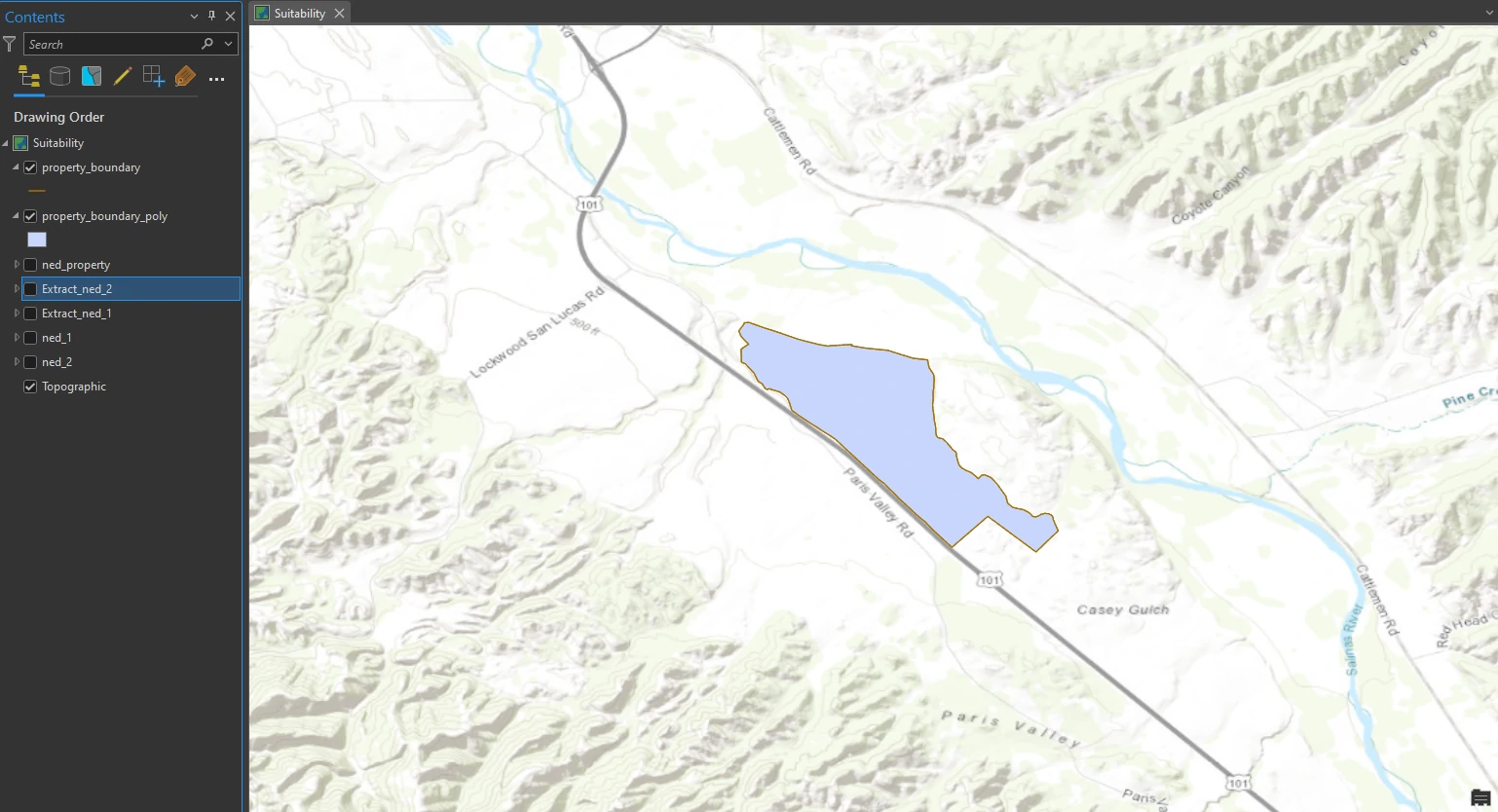
Convert a line feature to a polygon feature

The data comes with property_boundary line that demarcates the boundary of an approximately 1,100-acre property dedicated to viticulture. We will use the Extract by Mask tool to reduce the extent of the elevation layers to match the extent of the property boundary. However, to use the property boundary layer as a mask, it must be a polygon. Because it is currently a line feature, we must first convert it to a polygon.

This process can be done by Feature to Polygon tool in the Geoprocessing pane. The result of this process can shown at below image.

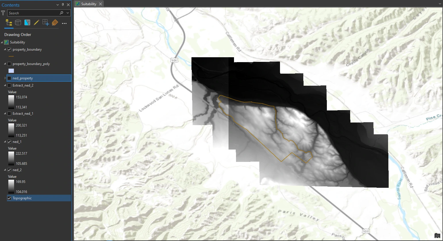
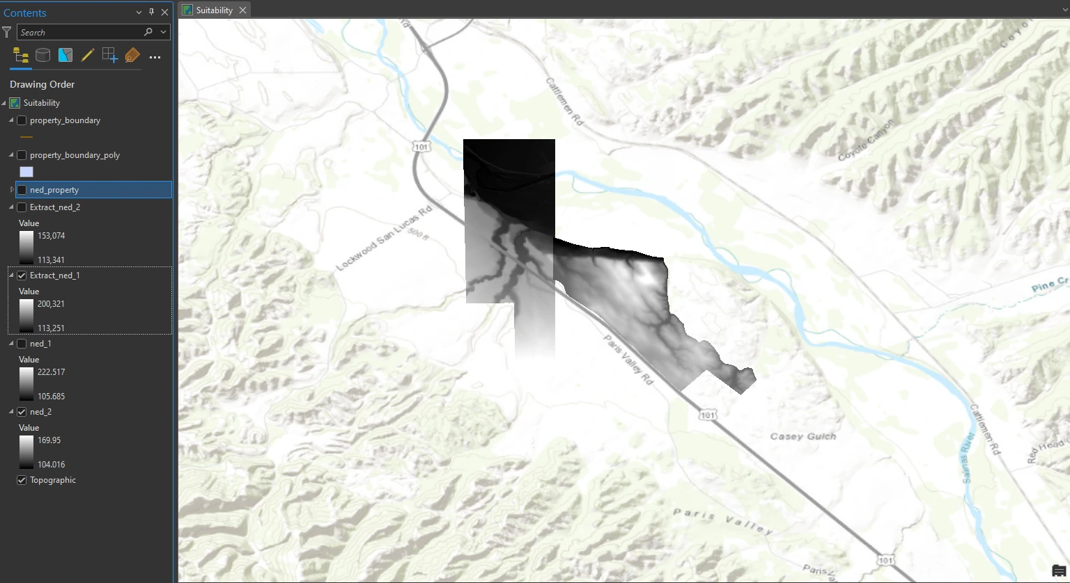
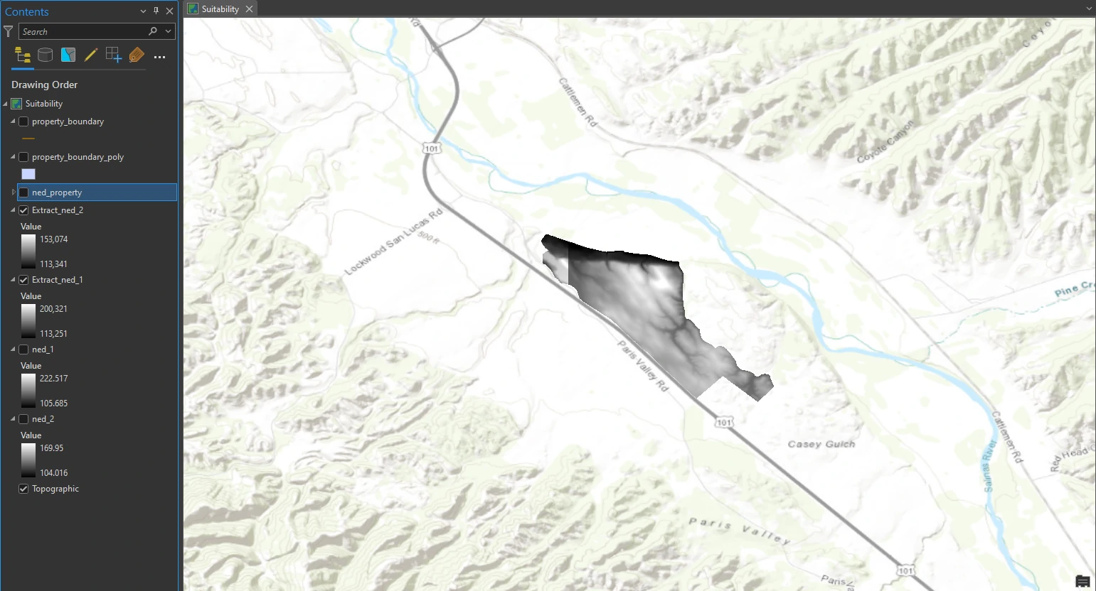
Clip raster layers

As you can see at the dataset image, the raster layer covering an area exceeding the limit of polygon boundary layer. To get more specific area inside polygon boundary, we can move forward with clipping the elevation rasters.

This process can be done by Extract by Mask tool in the Geoprocessing pane. The result of this process can shown at below image.

Merge rasters

Next, we will merge Extract_ned_1 and Extract_ned_2 into a new raster dataset so that we can run analysis operations once, not twice.

This process can be done by Mosaic to New Raster tool in the Geoprocessing pane. Make sure that using polygon boundary layer as Spatial Reference due to it has both a geographic and a projected coordinate system, so the result will more accurate and inherit both coordinate system. The result of this process can shown at below image.

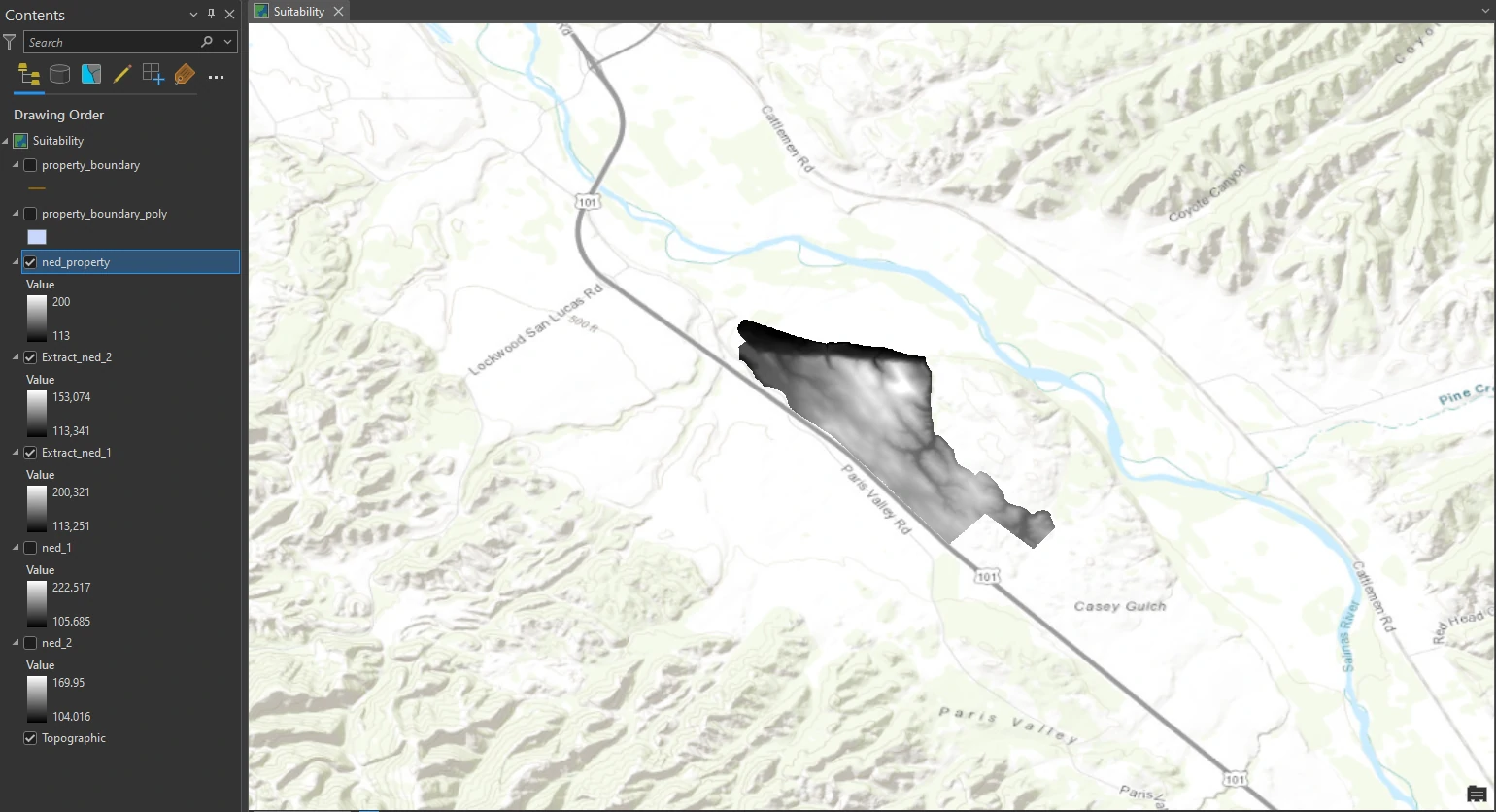
Our preprocessing is complete. One elevation raster is clipped to the extent of the study area and projected appropriately.

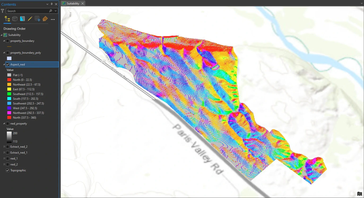
Derive an aspect surface

In this part we will create an aspect surface to determine which areas of the property are south facing (the preferred aspect for a vineyard). Analyze the aspect of the topography (ground surface relief) is process to determine which direction each part of the ground primarily faces—north, south, east, west, or in between.

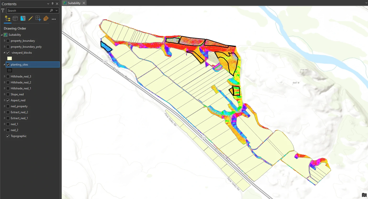
This process can be done by Aspect — the Spatial Analyst toolbox tool in the Geoprocessing pane. The result of this process can shown at below image. Notice the areas that face south, southeast, or southwest.

Derive a slope surface

Next, we will create a slope surface to determine which areas of the property have slope measurements of 14 percent or less (required for machine harvesting).

This process can be done by Slope — the Spatial Analyst toolbox tool in the Geoprocessing pane. By this tool we will set parameters as follow:

• Output Measurement = Percent Rise
• Maintain the Method and Z Factor as default value.

The result of this process can shown at below image.

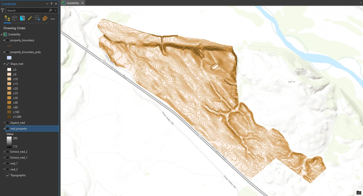
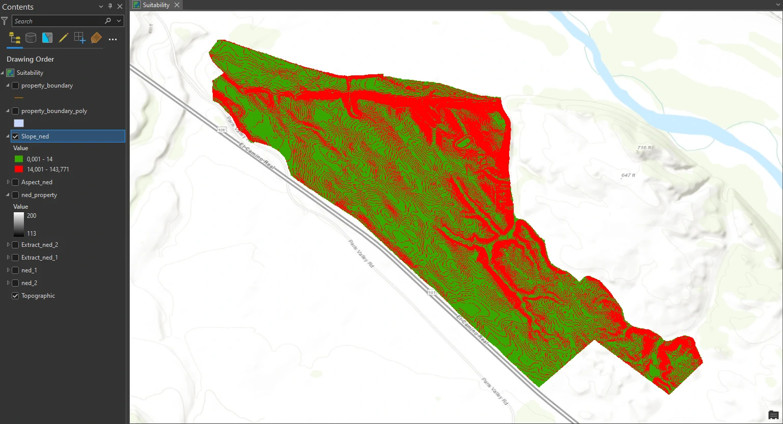
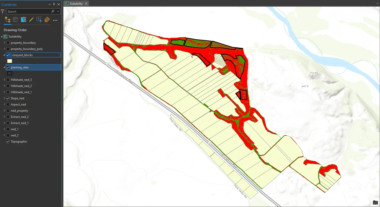
We are interested in seeing only whether the slope is less than or greater than 14 percent, so we will symbolize the layer for only these two categories. In the Symbology pane, change Method to Equal Interval and the number of classes to 2, change Method back to Manual Interval. Next, we change first Upper value box to 14.

We can see that although much of the property meets the criterion of having a slope that is less than or equal to 14 percent, a fair amount of it still has a greater percentage rise, which is not ideal for a new machineharvestable vineyard.

Derive a hillshade surface

A hillshade is a surface layer that depicts shadows to model the effect of an illumination source (usually the sun) over the terrain of the land. To create a hillshade, we must enter an azimuth and altitude value. Azimuth is the direction of the sun, expressed in positive degrees from 0 to 360, measured clockwise from north. Altitude is the angle of the sun above the horizon. The altitude is expressed in positive degrees, with 0 degrees at the horizon and 90 degrees directly overhead.

In other words, relative to any given surface,

azimuth tells us where in the sky the sun is altitude tells us how high.

These values change depending on the time of day and the time of year. By using these times, we can get the azimuth and altitude values, i.e. we can get those values from the US Naval Observatory Astronomical Applications Department.

Our criteria indicate that we want a lot of sun, especially during the critical fruit-ripening stage just before harvest. Harvest is usually sometime in October, depending on various factors.

For this project, we will set 2 values for the azimuth and altitude:

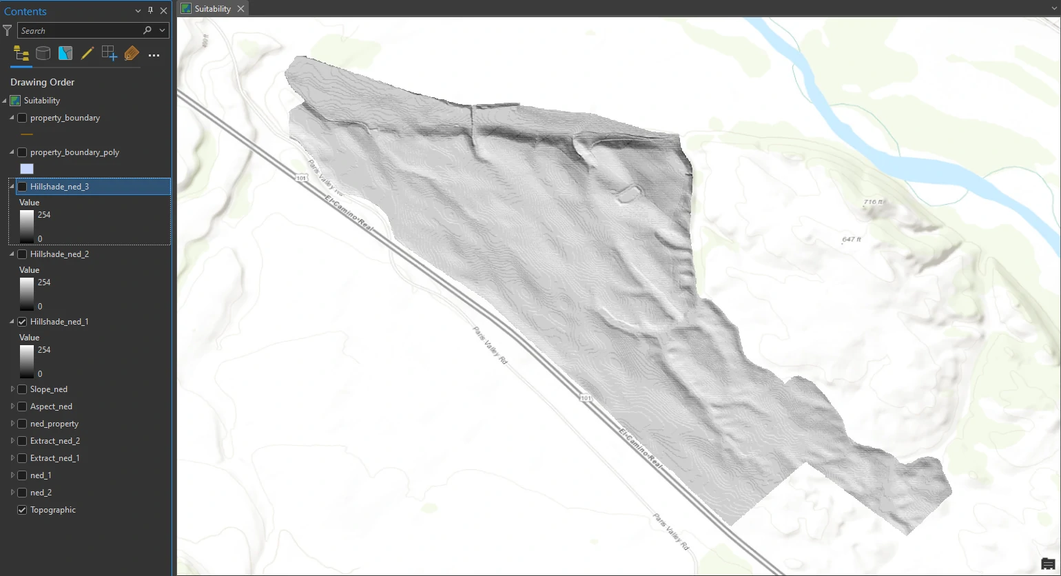
• Hillshade_ned_1 — at 2:00 p.m. in mid-September.
  • zimuth = 206.2
  • altitude = 53.9
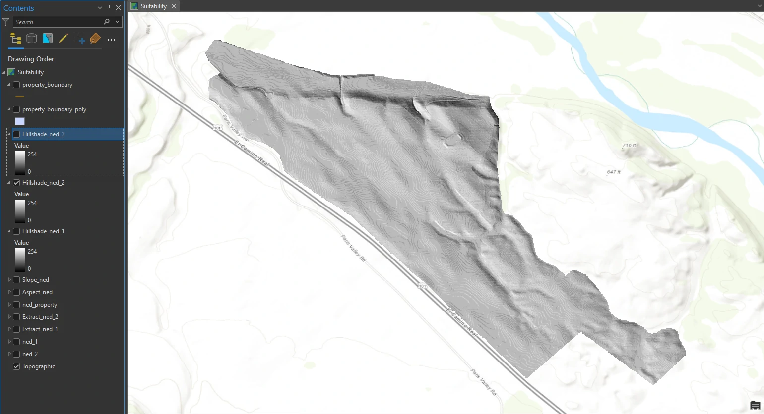
• Hillshade_ned_2 — at 3:00 p.m. in mid-September.
  • zimuth = 226.8
  • altitude = 46.6
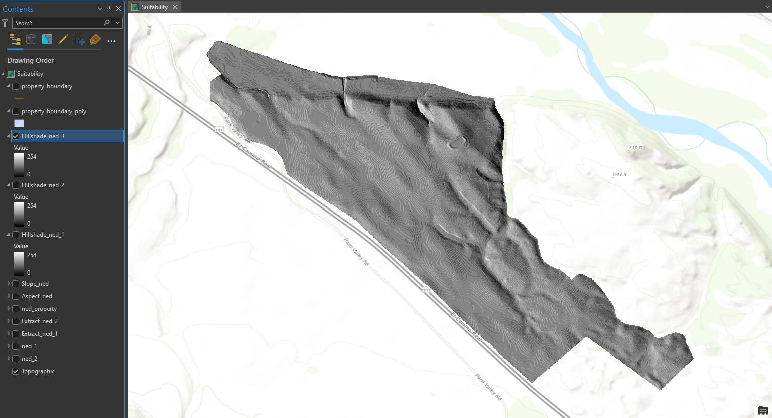
• Hillshade_ned_3 — at 4:30 p.m. in mid-September.
  • zimuth = 248.1
  • altitude = 31.3

The outputs are 3 shaded relief layers that shows which areas are illuminated and which are in shadow at respective time. A raster cell value of 0 represents complete shadow, with no illumination from the sun. A raster cell value of 255 represents full illumination.

Hillshade_ned_1

Hillshade_ned_2

Hillshade_ned_3

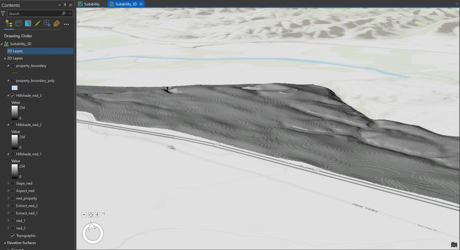
We can tilt out raster and render it into 3D to examine more the relief og this layer.

Visually compare analysis outputs

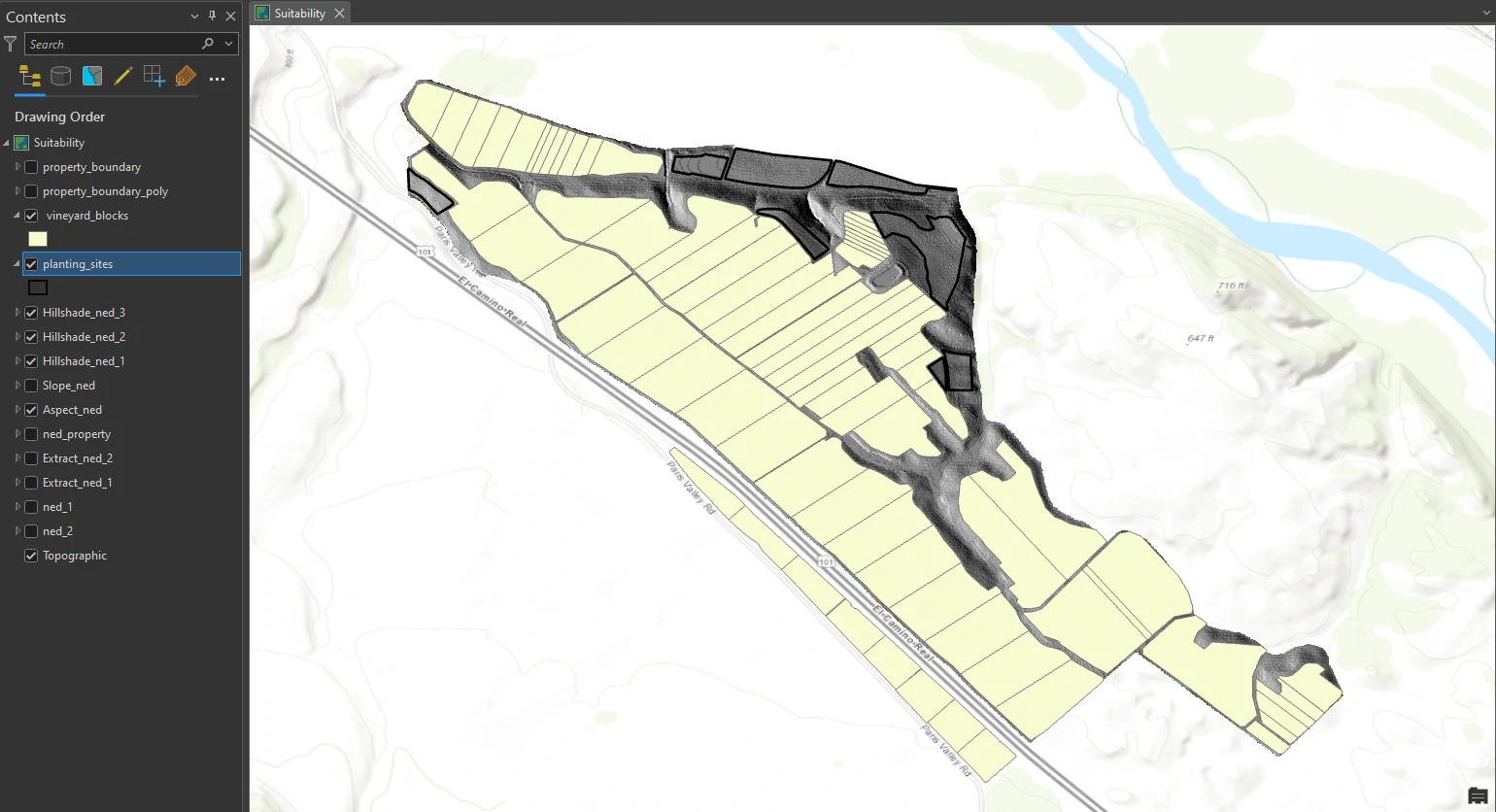
Finally we can stack these layers to get more information about our dataset. Here we combine vineyard_blocks, planting_site, and Hillshade_ned_3.

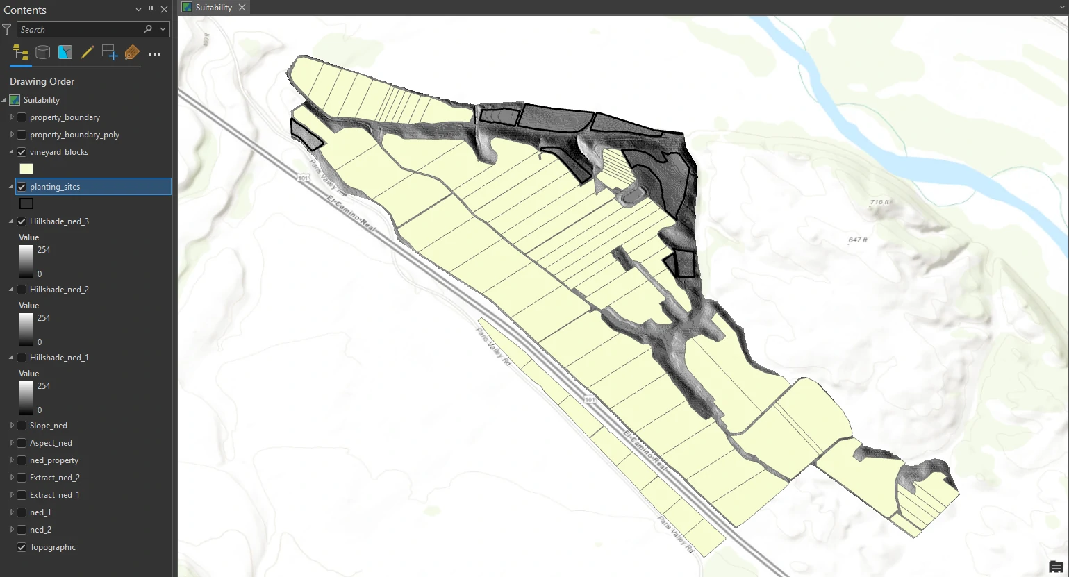
This layer represents already planted vineyard blocks. Next, we would typically hand-digitize a layer of potential planting sites using ArcGIS Pro editing tools and our knowledge of the property, but to save time, it will be provided. planting_site are unplanted areas of the property are available for future plantings. These areas have mostly low-slope land (a lot of green shading).

Create a weighted suitability model

We will find the most suitable planting site by combining the values of three layers (aspect, slope, and the third hillshade that shows sun illumination in the latest part of the afternoon).

Combining them as they are now would produce nonsensical results. Consider: How does a slope of 9 compare with a hillshade value of 190? Instead, we will reclassify the values so that we can add them together. (That means we will replace raster cell values with new cell values so that the rasters can be logically combined.) Each layer will be weighted—that is, as a percentage of the whole. In this way, we can prioritize our criteria. For example, if having the correct slope is most important, we will give slope the highest weight.

Reclassify criteria rasters

This part we will reclassify three criteria surfaces: Aspect_ned, Slope_ned, and Hillshade_ned_3. Replace the original cell values with either 1 (for desirable values) or 0 (for undesirable values).

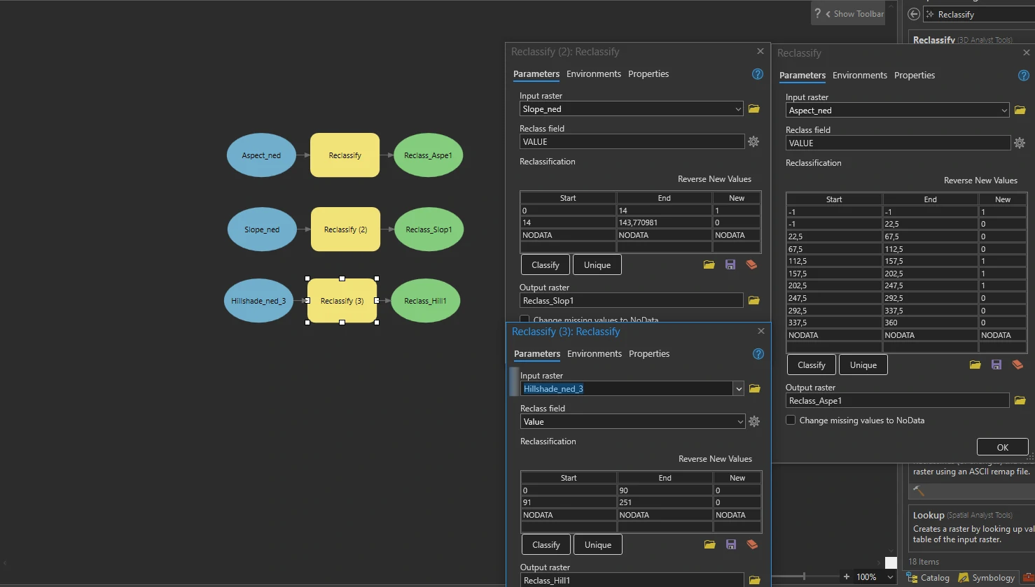
Next, we will use ModelBuilder and Reclassify tool on the Analysis tab to reclassified so that their cell values make sense in a calculation. In this case, we will change the desirable cell values to 1 and the undesirable values to 0.

By this tool we will set parameters as follow:

• For Input raster = Aspect_ned
  • Reclass Field = VALUE
  • Give the desirable traits (Flat, South, Southeast, and Southwest) a new value of 1 and the others a new value of 0. The desirable values are Southeast (112.5–157.5), South (157.5–202.5), and Southwest (202.5–247.5). We will also consider flat surfaces (−1) as desirable.
• For Input raster = Slope_ned
  • Maintain the other parameters, but for the 14–143.770981 category, change the New value to 0.
• For Input raster = Hillside
  • we want to rule out areas that have little to no sunlight. Knowing that 0 means no illumination and 251 is the highest level of illumination at this time of day (look at the legend), we decide to draw the “unacceptable” cutoff value at 90.
  • So we generate 3 classification with:
    • 0 — 90 = 0 or no illumination
    • 91 — 251 = 1 or illumination
    • NODATA

The result schema can we shown below.

Combine criteria rasters

Finally, we will Add a Raster Calculator process to the model. Add together the reclassified values of the three inputs but multiply each input by a percentage of 100. In this way, our end results will be weighted according to criteria priority.

This process can be done by Raster Calculator tool in the Geoprocessing pane (Spatial Analyst toolset).

We decide to weight aspect, slope, and hillshade to 20 percent, 50 percent, and 30 percent, respectively. By that weight we can input these number using expression box.

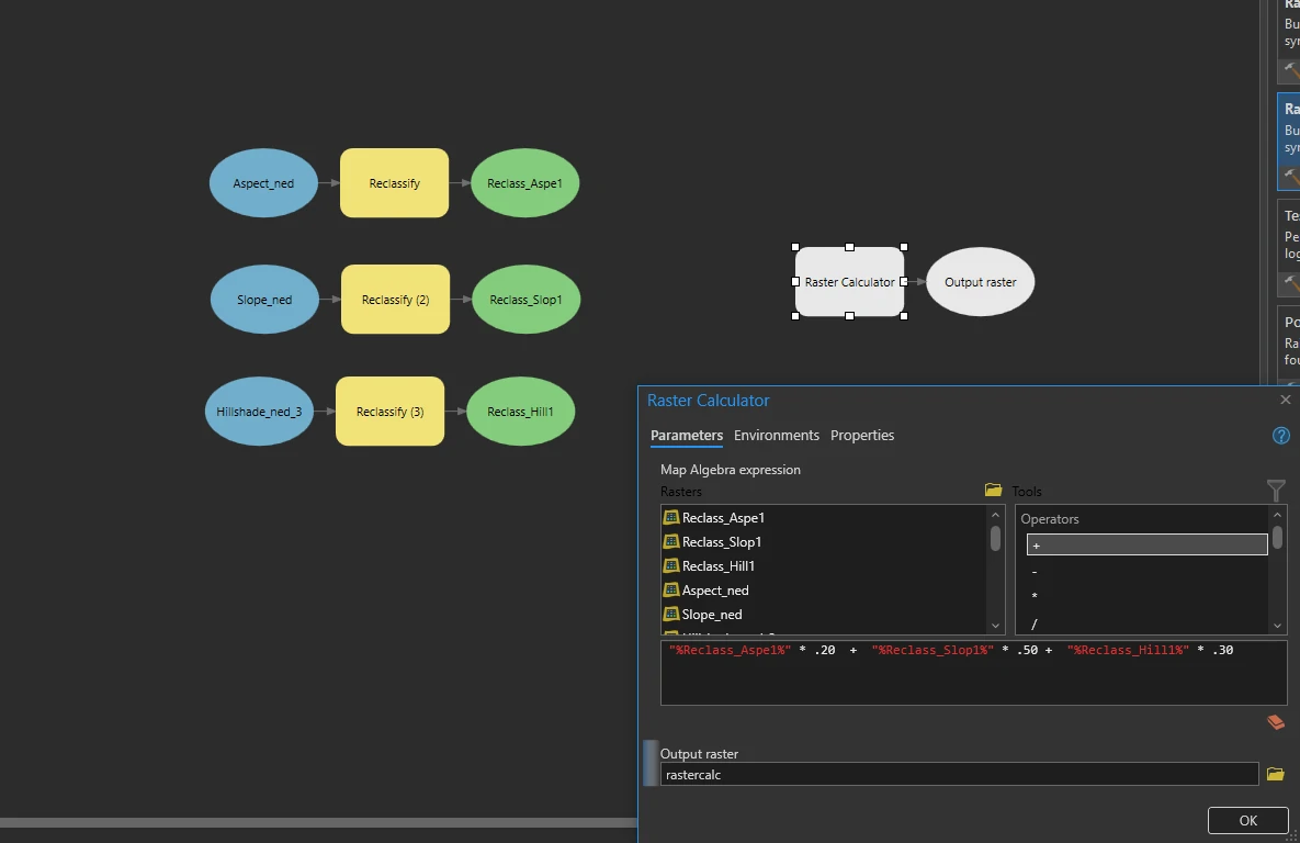
“%Reclass_Aspe1%” * .20 + “%Reclass_Slop1%” * .50 + “%Reclass_Hill1%” * .30

The final schema model can shown at below image.

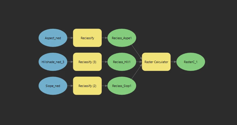
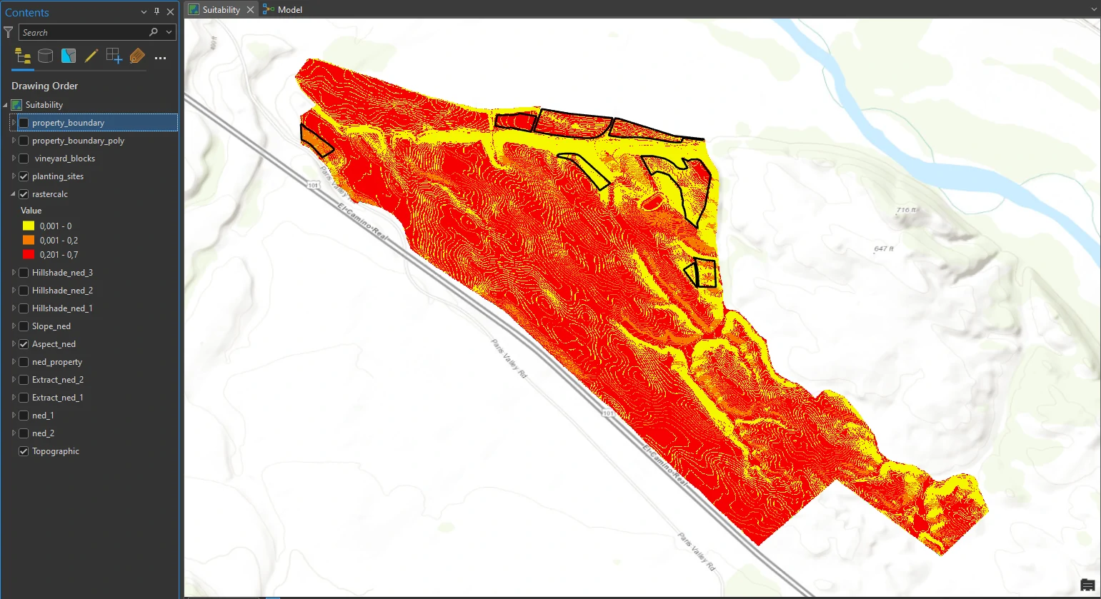
This process will return a calculated raster layer that contain result of reclassify and Combine criteria.

Areas of darker red indicate higher values from the raster calculation and the most desirable characteristics. The three areas at the top of the figure are the top three candidates.

This result can be one of decision process to determine most suitable area for planting additional vines. The GIS analysis is an important first step, but it is just one piece of the equation. We know that these sites are geographically suitable for planting, but now the owners must consider several other factors before investing in planting. i.e.:

• grape varietal
• the average tonnage yield per acre
• what is the average price per ton that they can expect to reap?
• How much will the additional vineyard blocks add to the overhead costs of fieldworkers, vineyard managers, fertilizer, water, pest abatement, and so on?
• Will the financial gain in good years be enough to offset losses from the inevitable challenges of drought, pests, or early frost?
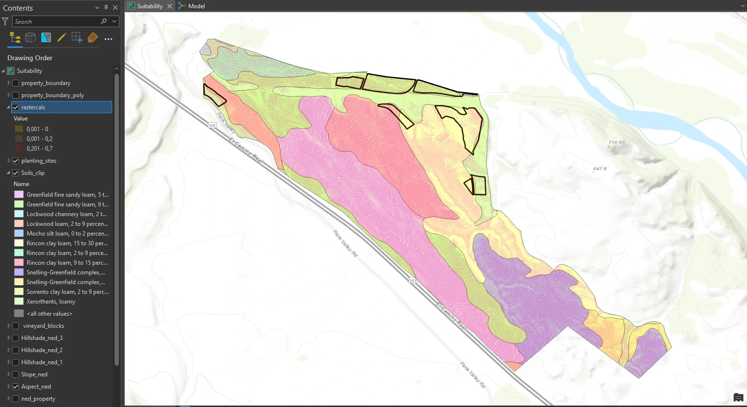
• What type of soil exists at each site, and how does that type affect the decision?

For the soil cases, we can deep dive about this issue by adding soil raster layer such as in this image below.