Voronoi diagram
geospatial
map
Estimating unknowns with spatial interpolation 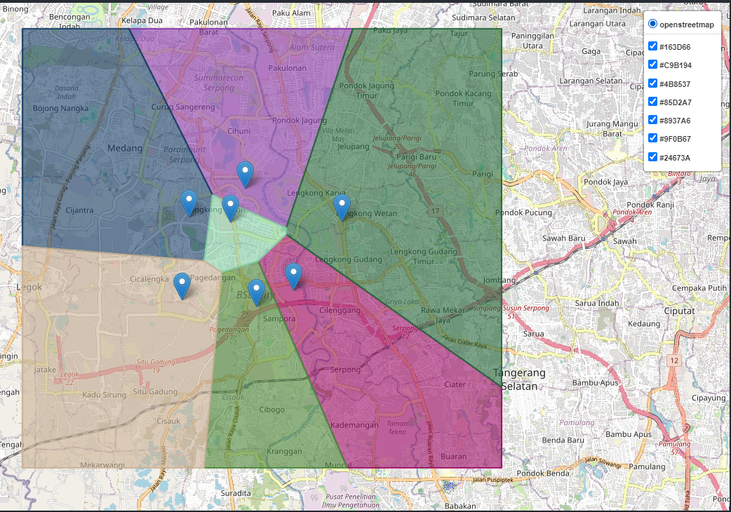
Introduction
Voronoi diagrams, named after the Russian mathematician Georgy Voronoy, are fascinating geometric structures with applications in various fields such as computer science, geography, biology, and urban planning. These diagrams provide a powerful tool for understanding spatial relationships and have become integral to computational geometry. In this article, we will explore the history, mathematics, construction methods, properties, applications, challenges, and implementation of Voronoi diagrams.
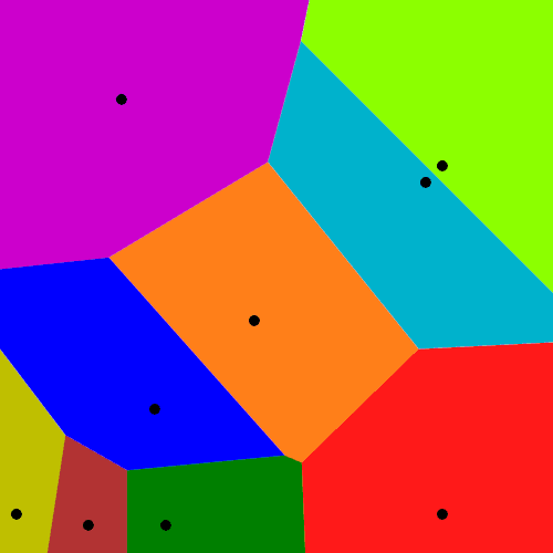
Suppose you have n points scattered on a plane, the Voronoi diagram of those points subdivides the plane in exactly n cells enclosing the portion of the plane that is the closest to the each point. For geospatial use case, it is useful to tell us the closest point of interest (POI) by representing each POI with a dot inside a polygon shape. So within a polygon, the closest POI is definitely the dot inside the polygon.
By using this diagram, we can make a region (or a cell) from a single point (let say it as * point) and define that in every point lies in that region, they have * point as a closest point of interest. So we can bring this concept to our business as: we can set up a warehouse’s location as a single point and create voronoi diagram to create coverage area for that warehouse and we can see how much customers inside coverage area and estimate how well that warehouse covering specific area for logistics plan.
Dataset
Load dataset
We’ll generate dummy dataset to create voronoi diagram
list_ = [
    Point(106.644085,-6.305286),
    Point(106.653261,-6.301309),
    Point(106.637751,-6.284774),
    Point(106.665062,-6.284598),
    Point(106.627582,-6.283521),
    Point(106.641365,-6.276593),
    Point(106.625972,-6.303643)
]

gdf = gpd.GeoDataFrame([[-6.305286, 106.644085], [-6.301309, 106.653261], [-6.284774, 106.637751], [-6.284598, 106.665062],
                        [-6.283521, 106.627582],[-6.276593, 106.641365], [-6.303643, 106.625972]],columns=["longitude","latitude"])

gdf['geometry'] = list_
gdf = gdf.set_crs("EPSG:4326")
The Code
By calling maps.voronoi_plot, we can generate geodataframe that contain voronoi diagram in polygon type. the data input only needs one geodataframe with geometry.
result = maps.voronoi_plot(gdf,geo_col='geometry', boundary=[106.619602,106.670929,-6.309795,-6.275227])
This function requires the following parameters:
- main_data (
geodataframe): Data location and value - geo_col (
string): geometry name column - boundary (
list):[min_longitude, max_longitude, min_latitude, max_latitude], 4 numbers that will generate boundary to limiting the voronoi diagram
The result
| index_left | longitude | latitude | geometry | colors | |
|---|---|---|---|---|---|
| 0 | 4 | -6.28352 | 106.628 | POLYGON ((106.586882 -6.2375029999999985, 106.61308380893126 -6.2375029999999985, )) | #163D66 |
| 1 | 6 | -6.30364 | 106.626 | POLYGON ((106.586882 -6.344376000000001, 106.586882 -6.290389924162609, )) | #C9B194 |
| 2 | 0 | -6.30529 | 106.644 | POLYGON ((106.63140819444598 -6.344376000000001, 106.63573922899768 -6.296629177824138, )) | #4B8537 |
| 3 | 2 | -6.28477 | 106.638 | POLYGON ((106.63573922899768 -6.296629177824138, 106.63145785535497 -6.2939565242581, )) | #85D2A7 |
| 4 | 5 | -6.27659 | 106.641 | POLYGON ((106.66777042545469 -6.2375029999999985, 106.65141445968877 -6.285921153748342, )) | #8937A6 |
| 5 | 1 | -6.30131 | 106.653 | POLYGON ((106.70415200000001 -6.344376000000001, 106.66647696627072 -6.344376000000001, )) | #9F0B67 |
| 6 | 3 | -6.2846 | 106.665 | POLYGON ((106.70415200000001 -6.2375029999999985, 106.70415200000001 -6.324724961342843, )) | #24673A |
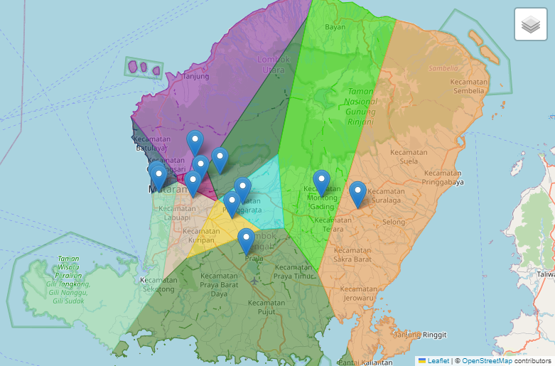
Real use case with voronoi diagram
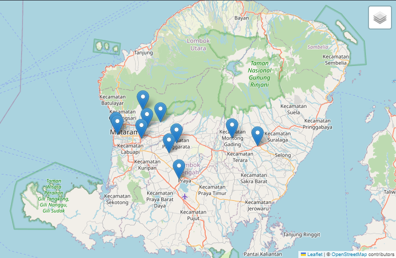
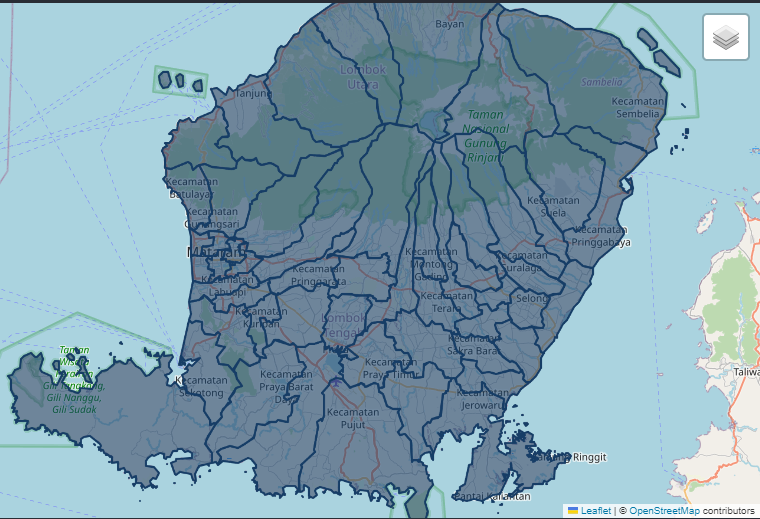
A Voronoi diagram helps us identify the nearest neighbor or determine the closest pair of points within a specific area. In this case, we’re focusing on Lombok, where we have several merchants who can assist with distributing our products. By using a Voronoi diagram, we can clearly see which merchant is closest to any given location, making it easier to plan and optimize our distribution.
Applications of Voronoi Diagrams in Various Fields
Voronoi diagrams have a wide range of applications in various fields. In computational geometry, they solve proximity problems, such as finding the nearest neighbor or determining the closest pair of points. In computer graphics and visualization, they generate realistic textures, simulate natural phenomena, and create visually appealing visualizations. Geographic information systems utilize Voronoi diagrams for spatial analysis, map overlay, and network planning. They play a crucial role in feature extraction, object recognition, and image segmentation in pattern recognition and image processing. Furthermore, Voronoi diagrams find applications in biology, physics, and urban planning.