Analyze Distance and Attractiveness using Huff models
geospatial
map
model
optimization
Imagine we deciding where to grab coffee. There’s a cozy café a block away with decent reviews, and a trendy one across town with killer lattes but a 20-minute drive. Which one do we pick?
This everyday decision —weighing convenience against appeal— is exactly what the Huff Gravity Model helps us quantify at scale.
Theory - What Is the Huff Gravity Model?
The Huff Gravity Model is a spatial probability model used in retail analytics and urban planning to estimate how likely someone is to visit a given location, like a store, bank, or service center. It considers two core ingredients:
- Attractiveness: How appealing is the destination?
- Distance: How far does a person have to travel to get there?
In simple terms, the model says:
The more attractive a location is, and the closer it is, the more likely people are to choose it over other options.
Here’s the basic formula:
\[P_{ij} = \frac{A_j / D_{ij}^b}{\sum_{k} A_k / D_{ik}^b}\]Where:
- \(P_ij\): Probability that a customer at location i visits store j
- \(A_j\): Attractiveness of store j
- \(D_ij\): Distance between i and j
- \(b\): Distance decay parameter (controls how strongly distance affects choice)
What Does “Attractiveness” Really Mean?
Attractiveness is where the Huff model gets interesting. It’s not a fixed concept — we define it based on what matters to our business. In another word, Attractiveness is a numerical score that represents how “desirable” or “competitive” a location is relative to others.
In a retail setting, attractiveness might include:
- Store size or layout
- Historical sales volume
- Product variety
- Brand reputation
- Customer ratings or reviews
- Affordability or pricing advantage (Lower price stores can be more attractive)
- Operating hours or Service Availability (Longer hours or more available services)
- Marketing presence (Heavy advertising can make a store more popular)
We can even use composite scores, combining multiple factors into one weighted value (weighted index from several metrics) that reflects how desirable a location is. The key is: what drives customer behavior in our market?
Example
Let’s say we have three stores:
| store_id | Size (sqm) | Monthly Sales | Brand Score | Attractiveness (Composite) |
|---|---|---|---|---|
| 1 | 500 | 100,000 | 80 | 0.5×Size + 0.3×Sales + 0.2×Brand |
| 2 | 600 | 90,000 | 90 | 0.5×Size + 0.3×Sales + 0.2×Brand |
| 3 | 400 | 120,000 | 70 | 0.5×Size + 0.3×Sales + 0.2×Brand |
We standardize and weight them accordingly, and use that score as \(A_j\) in the model.
We can also flip the concept—think about negative attractiveness. What might repel a customer? Poor parking? Long wait times? Weak brand perception? These factors can be integrated to lower a location’s score.
Tips When Choosing Attractiveness
- Make it consistent across all locations (e.g., don’t mix monthly and yearly sales).
- Normalize/scale if we’re combining multiple indicators.
- Use business intuition or statistical methods (e.g., PCA or regression) if we have historical choice data to back it up.
- Try testing different metrics and see which one gives results that match reality best.
Why Use the Huff Model?
- Smarter Site Planning By modeling customer choice behavior, we can:
- Identify underserved areas
- Evaluate where a new site should go
- Predict cannibalization between our own stores
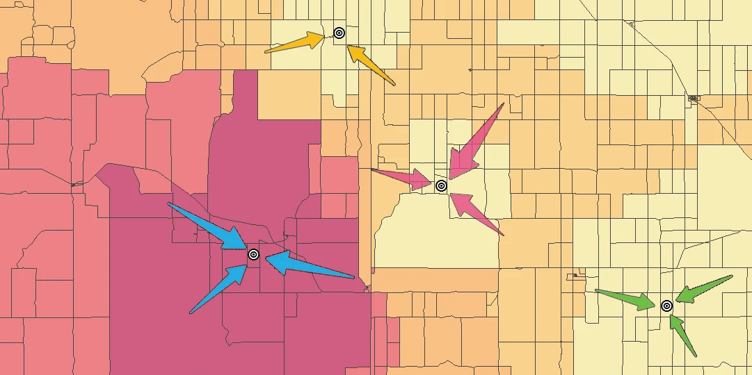
- Competitive Benchmarking Overlay Huff probabilities on a map to visualize customer draw zones — ours vs. competitors. See where we’re winning… and where we’re not.
- Impact Simulation Change an attractiveness variable — say, increase store size or extend hours—and rerun the model. we’ll instantly see how it shifts the probability of visits.
Implementing the Huff Model
To implement a Huff model using Python, we’d typically work with:
- GeoPandas & Shapely: to handle geographic data (e.g., store and customer locations)
- NumPy or Pandas: for calculations
- Rasterio or Matplotlib: to visualize the result as probability maps
- GIS tools (ARGIS Pro, QGIS, etc)
Here’s a simplified version of the process:
- Collect data: Store locations, attractiveness metrics, and consumer locations (e.g., population centroids)
- Calculate distances between each consumer and each store
- Compute probabilities using the Huff formula
- Aggregate or visualize results using maps or plots
Dataset
Load dataset
We will use atleast 2 datasets that contain:
- Center location - such as: store, bank, hospital, etc.
- Customer location
These dataset must have geographic coordinate (longitude and latitude) which used for distance calculation. In the code below, we will use sample data to show how to use this model.
stores = pd.DataFrame({
    'store_id': [1, 2, 3],
    'attractiveness': [100, 150, 120],
    'lon': [106.8, 106.9, 107.0],
    'lat': [-6.2, -6.25, -6.3]
})

customers = pd.DataFrame({
    'customer_id': ['A', 'B', 'C', 'D', 'E'],
    'lon': [106.85, 106.88, 106.95, 107.02, 107.1],
    'lat': [-6.22, -6.26, -6.27, -6.28, -6.35]
})

# Convert to GeoDataFrames
gdf_stores = gpd.GeoDataFrame(stores, geometry=gpd.points_from_xy(stores.lon, stores.lat), crs="EPSG:4326")
gdf_customers = gpd.GeoDataFrame(customers, geometry=gpd.points_from_xy(customers.lon, customers.lat), crs="EPSG:4326")
gdf_stores
| store_id | attractiveness | lon | lat | geometry | |
|---|---|---|---|---|---|
| 0 | 1 | 100 | 106.8 | -6.2 | POINT (106.8 -6.2) |
| 1 | 2 | 150 | 106.9 | -6.25 | POINT (106.9 -6.25) |
| 2 | 3 | 120 | 107 | -6.3 | POINT (107 -6.3) |
gdf_customers
| customer_id | lon | lat | geometry | |
|---|---|---|---|---|
| 0 | A | 106.85 | -6.22 | POINT (106.85 -6.22) |
| 1 | B | 106.88 | -6.26 | POINT (106.88 -6.26) |
| 2 | C | 106.95 | -6.27 | POINT (106.95 -6.27) |
| 3 | D | 107.02 | -6.28 | POINT (107.02 -6.28) |
| 4 | E | 107.1 | -6.35 | POINT (107.1 -6.35) |
The Code
By calling maps.huff_gravity_model, we can calculate distance and apply Huff gravity model. The output of this function is a tabel that show how likely someone is to visit a given location and it distance to that location.
result = maps.huff_gravity_model((main_data, mass_center, col_list=[], target_name=['mass_center','small_obj', 'target'], dist_decay=2, dist_type='euclidean', distance_data=None))
This function requires the following parameters:
- main_data (
geodataframe): Data customer location and value - mass_center (
geodataframe): Data for given location and value - col_list (
list): list columns that contain of geographic coordinate - target_name (
list): list of ID and attractiveness columns - dist_decay (
int): Distance decay parameter (controls how strongly distance affects choice) - dist_type (
string): type of distance that we want to measure. - distance_data(
list): provided distance between costomer and locations (optional).
The result
| store_id | customer_id | probability | distance | |
|---|---|---|---|---|
| 0 | 1 | A | 0.416628 | 5.9592 |
| 1 | 1 | E | 0.0658894 | 37.1108 |
| 2 | 1 | C | 0.0402481 | 18.3161 |
| 3 | 1 | B | 0.0315 | 11.0638 |
| 4 | 1 | D | 0.0112834 | 25.9038 |
| 5 | 2 | B | 0.94488 | 2.4741 |
| 6 | 2 | C | 0.570427 | 5.9587 |
| 7 | 2 | A | 0.533189 | 6.4516 |
| 8 | 2 | E | 0.222394 | 24.7396 |
| 9 | 2 | D | 0.060621 | 13.6873 |
| 10 | 3 | D | 0.928096 | 3.1288 |
| 11 | 3 | E | 0.711717 | 12.3693 |
| 12 | 3 | C | 0.389325 | 6.4512 |
| 13 | 3 | A | 0.0501824 | 18.8095 |
| 14 | 3 | B | 0.0236204 | 13.9961 |
From table above, we can get each store and customer and probability of someone to visit a given location and it distance to that location, we add distance for each row to give us more understanding about probability result.
Conclusion
The Huff Gravity Model takes the guesswork out of understanding where our customers go—and why. It turns distance and appeal into data, helping us visualize competition, improve customer reach, and make confident decisions about new locations or investments.
As customers continue to choose between convenience, quality, and brand loyalty, the Huff model gives us a framework to simulate and optimize how our physical presence aligns with their preferences.