The H3 spatial index
geospatial
map
index
A discrete global grid system for indexing geographies into a hexagonal grid.
Introduction
The Hexagonical Hierarchical (H3) index was developed by Uber to help it analyze supply and demand within its ride-sharing marketplace efficiently and to help it optimally price its services. Uber released H3 to the public under an open source license in 2018.
The H3 grid system comprises nesting hexagons that cover the Earth’s surface. There are a total of 16 resolutions of the H3 grid system, with the first level containing 122 hexes and the 16th level containing over 569 trillion unique hexes. The area of the hexes in each level gets progressively smaller and is 1/7th the size of the hexes in the prior level. For each resolution, the hexes are assigned unique identifiers that can be appended to other geographic data to aid in efficient spatial analysis and feature engineering.
Advantage
- Help to organize the planet so we can measure, comapre, and analyze it.
- Covering the surface with perfectly fitting shapes that don’t overlap or leave gaps.
- Uniform shape
- Uniform edge length
- Uniform angles
- More natural neighbourhoods - every cell has 6 equal neighbours — More consistent distances - No long diagonal weirdness like squares. — More efficient space-filling - less over/under coverage
- It breaks the world into 15 resolutions, from country-sized hexagons to tiny ~1 cm² cells.
- It’s hierarchical — Big hexagons contain smaller ones, all the way down.
- It’s consistent — the same rules apply everywhere on Earth.
Reference
we encourage you to read Uber’s blog post at https://www.uber.com/blog/h3/.
Dataset
Load dataset
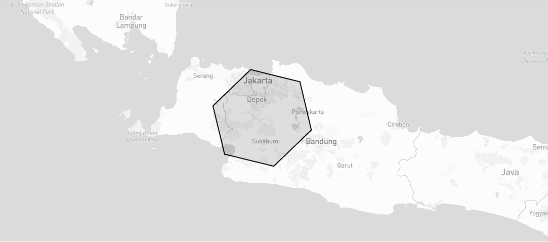
First, we load two datasets. Overal, there datasets contain the names of locations in New York, location code, Shape length, Shape area, and their cordinates.
these dataset have difference type:
- Polygon / multipolygon geometry dataset
- point geometry dataset
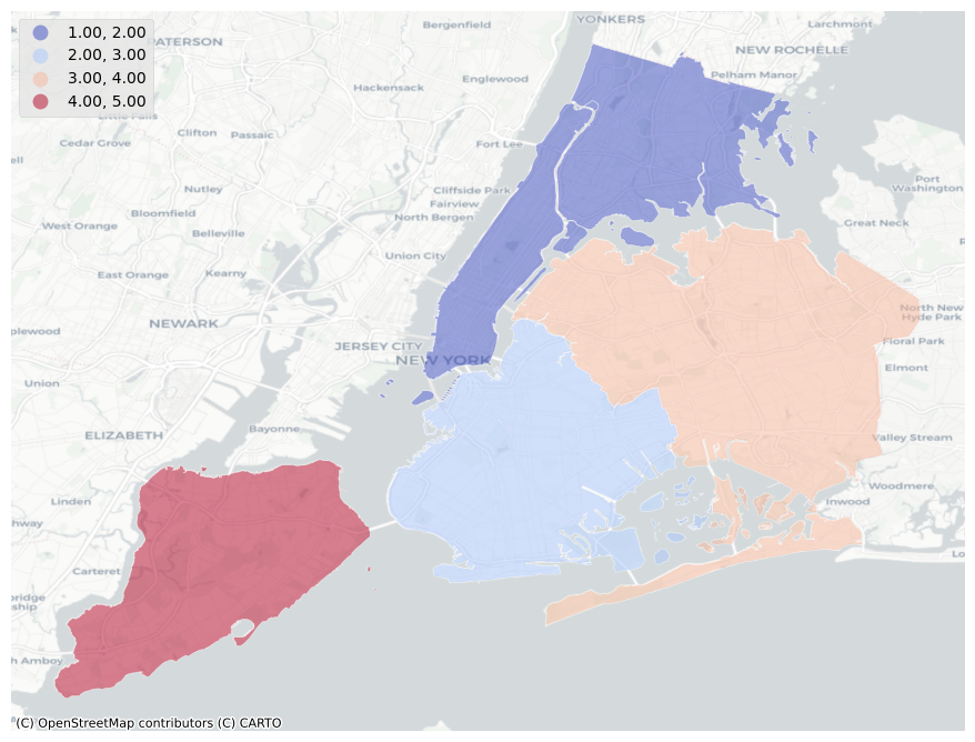
Load Polygon data
df = gpd.read_file('zip:///../map/book/nybb_16a.zip!nybb_16a/nybb.shp')
df = df.to_crs(epsg=4326)
| BoroCode | BoroName | Shape_Leng | Shape_Area | geometry | |
|---|---|---|---|---|---|
| 0 | 5 | Staten Island | 330470 | 1.62382e+09 | MULTIPOLYGON (((-74.05051 40.56642, -74.05047 |
| 1 | 4 | Queens | 896344 | 3.04521e+09 | MULTIPOLYGON (((-73.83668 40.59495, -73.83678 |
| 2 | 3 | Brooklyn | 741081 | 1.93748e+09 | MULTIPOLYGON (((-73.86706 40.58209, -73.86769 |
| 3 | 1 | Manhattan | 359299 | 6.36472e+08 | MULTIPOLYGON (((-74.01093 40.68449, -74.01193 |
| 4 | 2 | Bronx | 464393 | 1.18692e+09 | MULTIPOLYGON (((-73.89681 40.79581, -73.89694 |
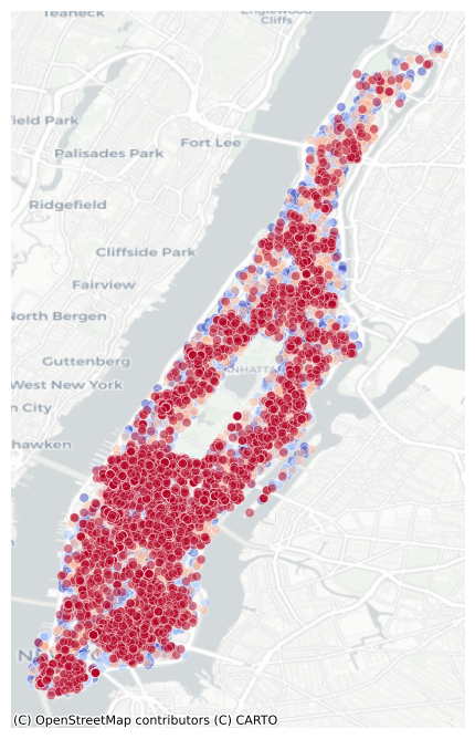
Load Point data
listings = pd.read_csv('../map/book/listings.csv')
listings_gpdf = gpd.GeoDataFrame(listings,
                        geometry=gpd.points_from_xy(listings['longitude'], listings['latitude'], crs="EPSG:4326")
)

boroughs = gpd.read_file(r"..\map\book\nybb.shp")
boroughs = boroughs.to_crs('EPSG:4326')
manhattan = boroughs[boroughs['BoroName']=='Manhattan']
listings_mask = listings_gpdf.within(manhattan.loc[3, 'geometry'])
listings_manhattan = listings_gpdf.loc[listings_mask]
| id | name | geometry | |
|---|---|---|---|
| 0 | 2595 | Skylit Midtown Castle Sanctuary | POINT (-73.98559 40.75356) |
| 2 | 6872 | Uptown Sanctuary w/ Private Bath (Month to Month) | POINT (-73.94255 40.80107) |
| 3 | 6990 | UES Beautiful Blue Room | POINT (-73.94759 40.78778) |
| 8 | 9357 | Midtown Pied-a-terre | POINT (-73.98664 40.76724) |
| 11 | 12192 | ENJOY Downtown NYC! | POINT (-73.98383 40.72296) |
The Code
By calling maps.geo_to_hexagon, we can convert geometry from specific dataset into a hexagonal grid.
result = maps.geo_to_hexagon(main_data, types='points', res=9, agg_col=None)
This function requires the following parameters:
- main_data (
geodataframe): Data location and value - types (
string): type of conversion (points, poly) - res (
int): resolution value of Hexagon - agg_col (
string): column name for aggregation from points to hexagon
The result
Polygon to hexagon

Point to hexagon
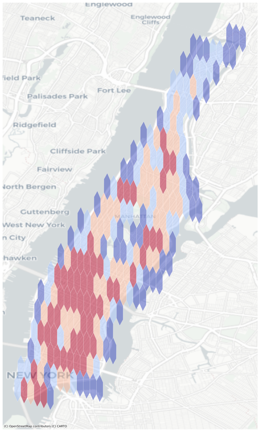
This process that convert polygon and points geometry to hexagon, help us to enables a range of algorithms and optimizations based on the grid, including nearest neighbors, shortest path, gradient smoothing, and more.