Geo-enabling data - geocoding

arcgispro

geospatial

map

esri

In ArcGIS Pro, we can also create features from information that describes or names a location—typically an address—through a process called geocoding. In some cases, we are often faced with situations in which data is not readily available. One of the advantages of geocoding is the ability to quickly create data from a list of points of interest that we have collected or researched.

We need several components to geocode addresses:

• An address table—a list of addresses for features that we want to map and that are stored as a database table or a text file
• Reference data—commonly from a street layer, on which the addresses can be located
• An address locator—a file that contains the reference data and various geocoding rules and settings

The ArcGIS Pro geocoding service uses address information in the attribute table of the reference data to calculate where addresses from the address table are located and creates points at those locations. As with other GIS data, the higher the quality of the reference data, the more accurately addresses can be geocoded. Ideally, street-level reference data includes attributes such as street name, street type, postal or zip code, and directional prefixes and suffixes to avoid ambiguity in address locations. And each street is divided into line segments that have starting and ending address numbers so that we can determine separate address ranges for each side of the street.

You can read more about Geocoding process using python — check out the full guide on this page

Study case scenario

Deciding on a retail site location is one of the most critical decisions a business must make. The success of the store depends on many factors related to location and demographics, such as access to potential and existing customers, visibility in its neighborhood, and appeal to its targeted audience, as well as wider demographics to catch potential consumers. we as an analyst who will prepare geographic and demographic data for use in support of a high-end bicycle retail site location and consultation service.

The Dataset

We will use RetailSiteStudy.gdb that contains:

• Bike Stations—a point feature class showing bike stations (Source: City of Houston)
• Existing Bike Lanes—a line feature class of existing bike lanes (Source: City of Houston)
• Proposed Bike Lanes—a line feature class of proposed bike lanes (Source: City of Houston)
• Commercial Land Use—a polygon feature class derived from a large land-use dataset (Source: City of Houston)
• Census Block Demographics—a polygon feature class of census block groups in the city of Houston (Source: City of Houston)
• Median household income (2010 census)—a table le that contains median household income values at the census block level for the city of Houston (Source: US Census Bureau, City of Houston)
• Roads—a line feature class (Source: City of Houston)
• retail_site_prospects—a text le that contains a compiled list of commercial properties.

Joining table

US Census data is a reliable and helpful resource for any research project that involves looking at demographic data and is collected with geographic detail that ranges from fine to general granularity. Almost all the data is stored as values in tables and not geoenabled. However, we can perform several steps to turn this data into a map.

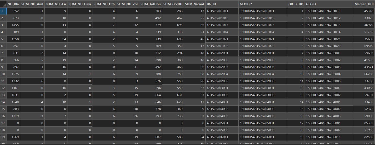
From Median household income table, first we can examine the columns GEOID and Median_HHI. The GEOID name is a standard identifier that the US Census Bureau provides to identify census blocks (a division of a census tract). The Median_HHI column represents median household income (in US dollars). This will be one factor in our decision-making process to determine a potential site for a retail location.

By using GEOID, we can join it to the city of Houston census block layer to make the information spatial. To do this we can go to attribute table pane options menu, point to Joins and Relates, and click Add Join.

Symbolize using graduated colors

With median household income added for each census block, we will now visualize the median household income with graduated colors on the map. This will be one factor of consideration when doing the analysis for prospecting a retail site location.

The median household income categories are as follows:

• Low Income: Less than $38,750
• Moderate Income: $38,751 to $63,250
• Moderately High Income: $63,251 to $ 97,800
• High Income: $97,801 to $156,950
• Very High Income: $156,951 to $250001

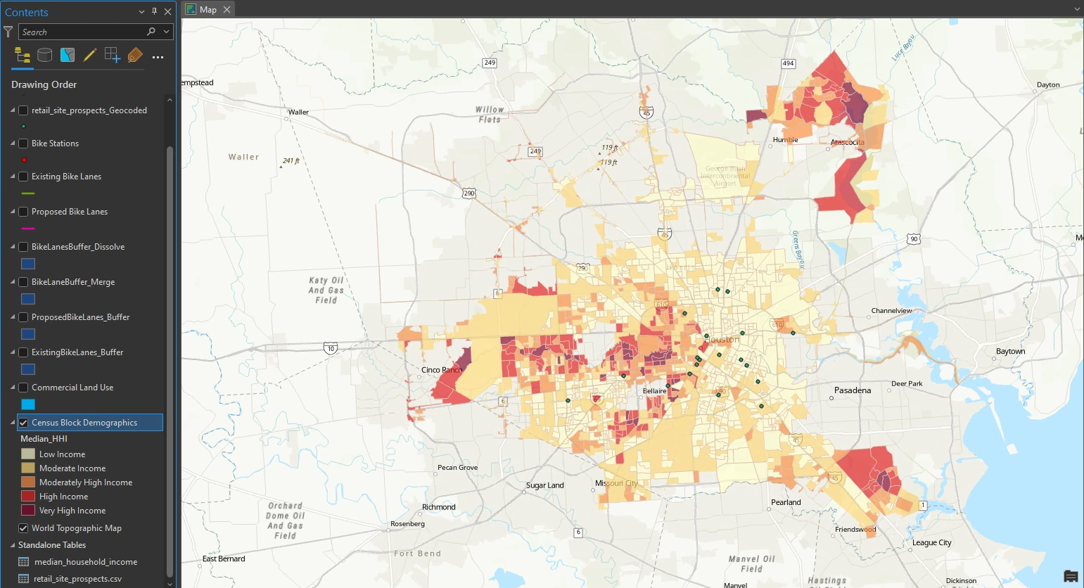
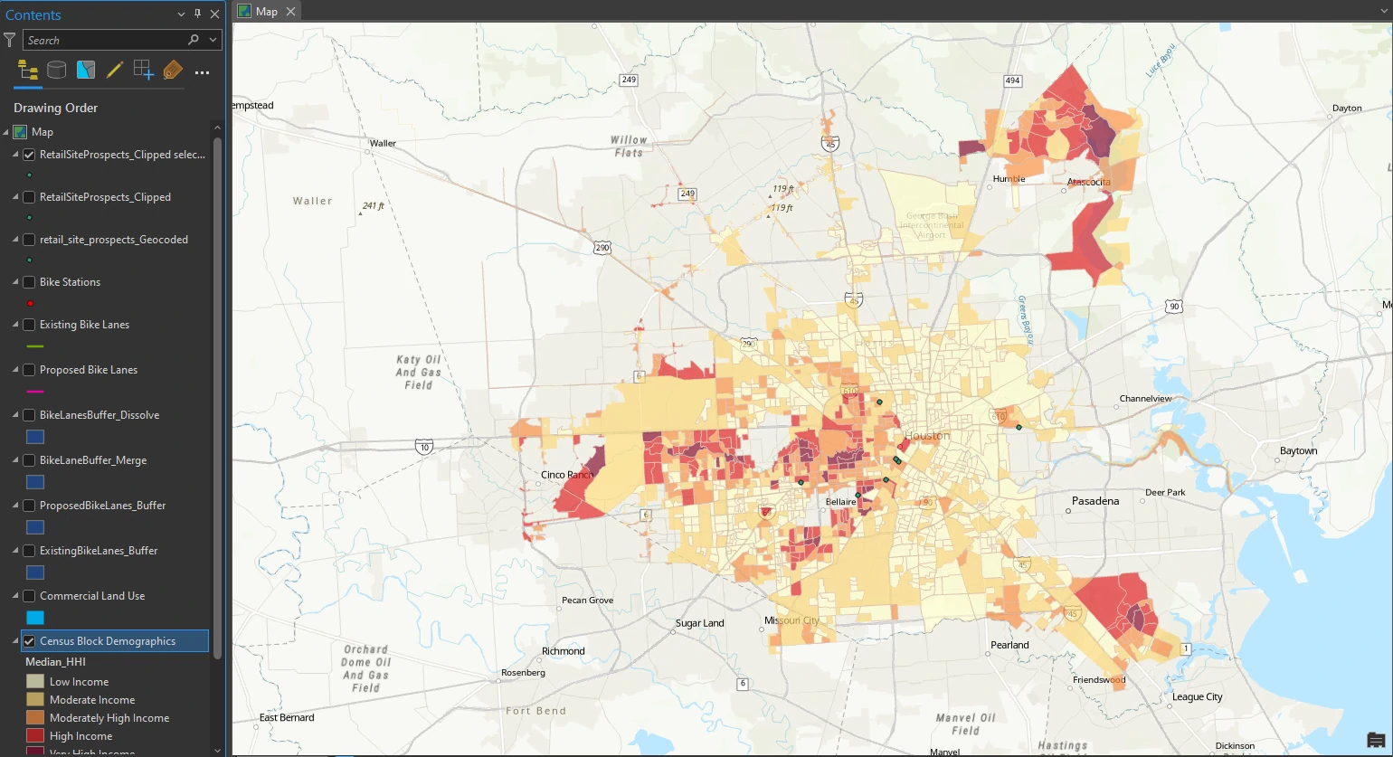
We can categorize this data by selecting Graduated Colors for Median_HHI columns with Manual Interval at symbology pane. Choose Orange-Red (5 Classes) from the Color Scheme list. and manually input upper value for each categories based on above information.

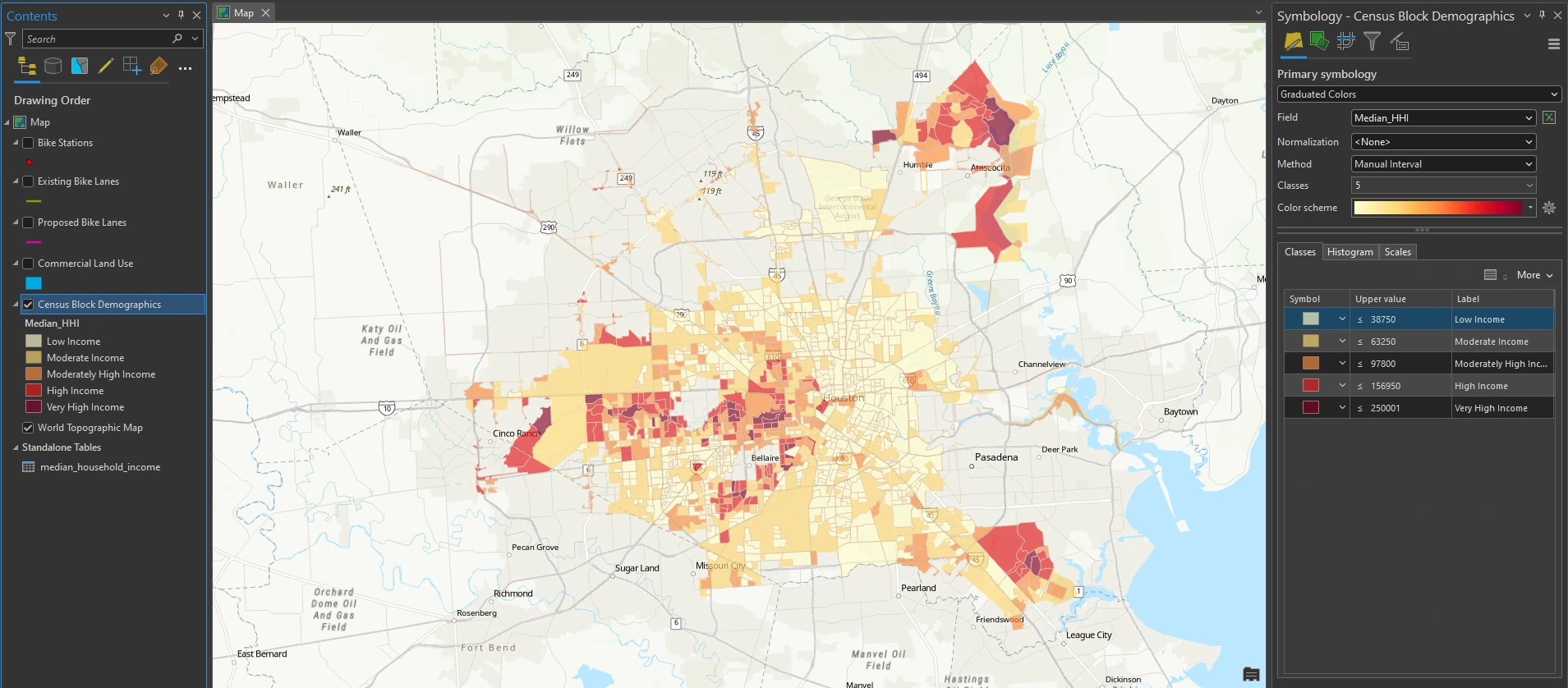
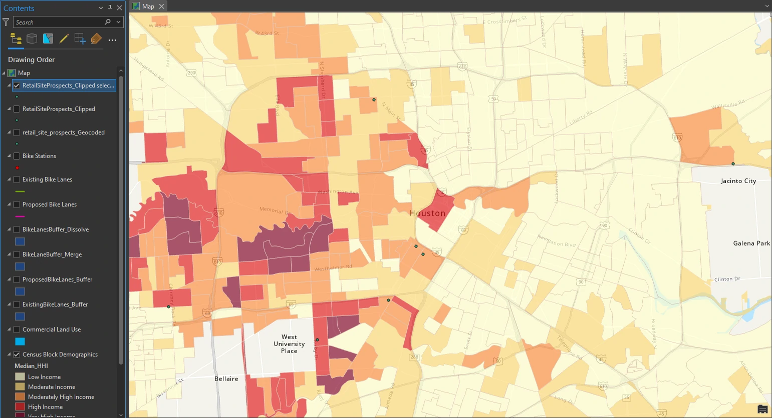
A color scheme is now applied so that we can visualize the areas that have differing levels of median household income. Moderate to very high-income areas are symbolized with gradually darker shades of orange-red and become emphasized. We can see areas on the west side of Houston and across a band through the center that have higher median household incomes that may support a large retail location (but may also be more expensive). Some census tracts may not have any symbology, which is often the case for areas designated as parks, airports, or port lands.

Geocode location data

A GIS must know two main pieces of information: the address of the business or home and knowledge of or reference to where that address is, such as street, main intersection, or neighborhood to easily find a location of a business or home and create address points. The process of creating map features from addresses, place-names, and similar information is called geocoding.

The process of creating map features from addresses, place-names, and similar information is called geocoding.

For our bicycle retail site location project, prospective retail locations are provided and must be geocoded — we must add a plain text file with addresses, names, and other information to our map. We will use a city of Houston street layer as the reference data — the spatial data that contains information about all the addresses.

When we geocode the table of retail locations, we will use the reference data to create an address locator to create point features that represent the locations of the addresses (also known as locator styles). When geocoding our table of addresses, the address compared with the address locator.

Create an address locator

An address locator defines which reference data will be used to search for addresses, which elements of the reference data will be searched against, and what format the address data will use. ArcGIS Pro comes with predefined locator roles that we can use to create locators. A role includes the elements of the address that are present (such as street name, number, direction) and the elements that will be used to locate our addresses.

Each locator role is unique and has specific requirements regarding the reference data it can use to match the format of addresses being geocoded. Some locators have more requirements than others, which allows for a wide range of accepted address formats. Using the appropriate role depends on knowing what type of reference data we have and what format our addresses will use.

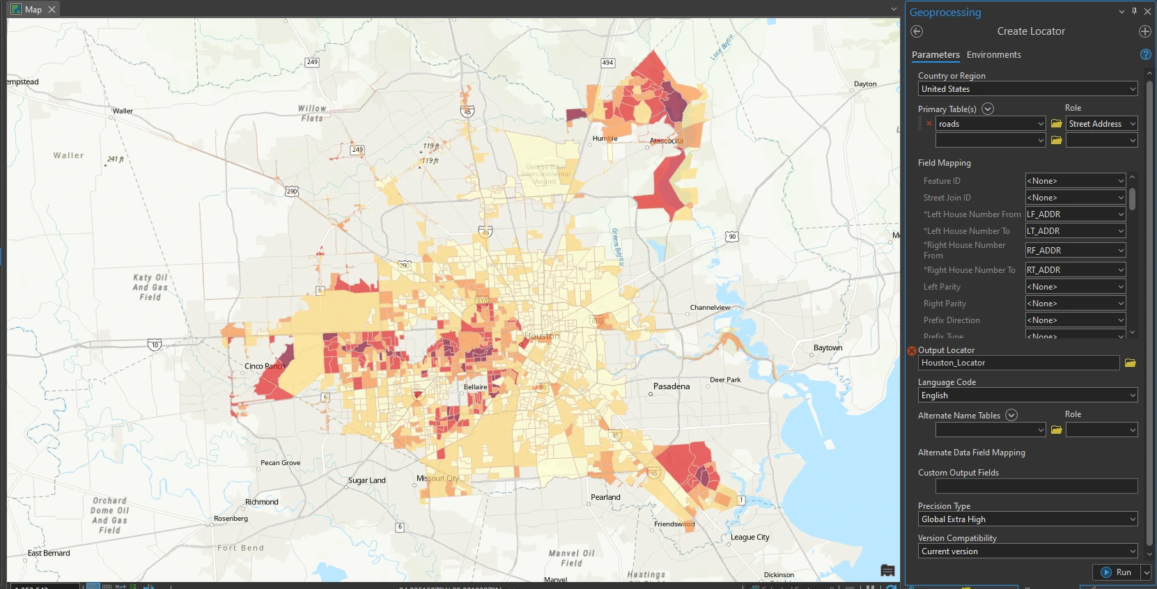
By utilize Create Locator tool at Geocoding Tools toolbox, we can create locator and setting these parameters=

• The Country or Region = United States
• Primary Tables = the roads layer in the RetailSiteStudy geodatabase
• Role = Street Address
• Left House Number From = LF_ADDR
• Left House Number To = LT_ADDR
• Right House Number From = RF_ADDR
• Right House Number To = RT_ADDR
• Street Name = NAME
• Left City = CITY_L
• Right City = CITY_R
• Left State = STATE_L
• Right State = STATE_R
• Left ZIP = ZIP_L
• Right ZIP = ZIP_R
• Output Locator = Houston_Locator

The roads layer acts as the reference data and it is assigned the role of Street Address. This layer has attributes for each street segment that indicate the range of addresses found on it. When we geocode an address, the address location is interpolated from the range of addresses found for a given segment.

In the Catalog pane, expand the Locators folder to verify that the locator was added.

The other address locator — ArcGIS World Geocoding Service — is included with ArcGIS Pro and is configured to help us locate places on a map in situations in which we may not be able to create our own. A locator also determines other settings for geocoding, including what makes up a matched address, search parameters, and tolerance for spelling errors.

Geocode addresses

Now that the locator is ready, the next step is to geocode the list of prospective retail sites. The output of the geocoding process can be either a shapefile or a geodatabase feature class of points. The geocoded data has all the attributes of the address table; some attributes of the reference data; and some additional attributes, such as the x,y coordinates of each point.

After we create address locator, we can make a geocode table from features table. Right-click ke table, and click Geocode Table. In the Geocode Table pane, read the guided workflow, scroll down, and click Go to Tool.

we apply there parameters to our Geocode Table pane:

• Input table = retail_site_prospects.csv
• Input Locator = HoustonLocator
• Output Feature Class = retail_site_prospects_Geocoded

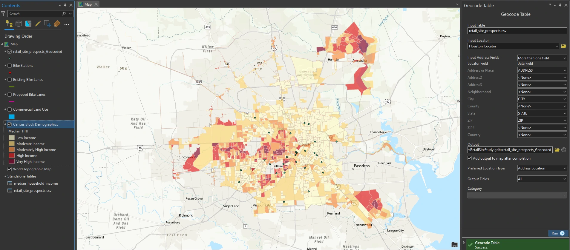
A dialog box appears that shows what addresses from the retail site prospects table are matched, unmatched, and tied with the roads data. All but three addresses are matched. we will perform an address rematch in the next step.

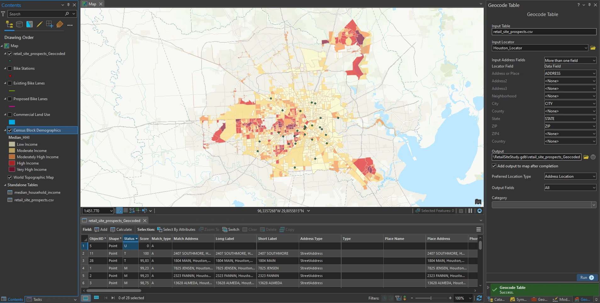
As a result of the geocoding, several additional attributes are added. The Status attribute column tells us whether each address is matched (M), unmatched (U), or tied (T). The Score attribute column tells us how well it scores when comparing the table with the reference data. The Match_type attribute shows how an address was matched—in this case, automatically (A) matched. The Match_addr attribute shows the actual address to which the retail site was geocoded, and the Side attribute tells us whether an address is on the right or left side of the street. The original fields of the table are preserved.

Rematch addresses

It is good practice to review all geocoded addresses and go through the address rematching process to ensure that the geocoded addresses are correct. Several retail site prospects were not properly geocoded—it could be due to incorrect address data or addresses that were geocoded to the wrong location. We will use the Rematch Address feature to identify the unmatched addresses and look at the tied addresses to interactively rematch them.

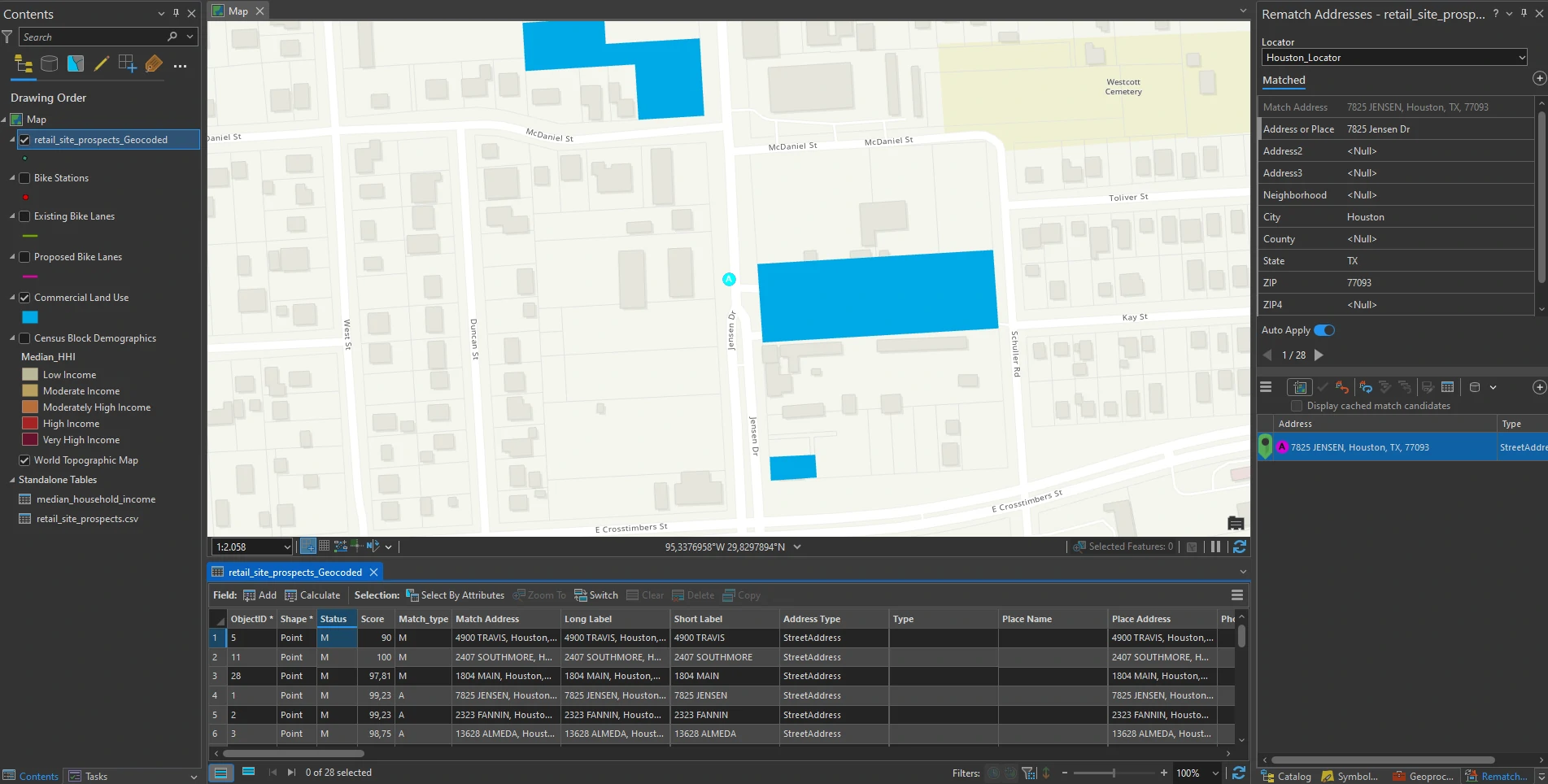
Right-click the result of the geocoding, click Data > Rematch Addresses to open the Rematch Addresses pane. The Rematch Addresses pane allows you to review which addresses are unmatched or insufficiently matched, and then go through the parameters for each address and adjust them to make a match.

The Rematch Addresses pane displays an address that is unmatched, Matched and Tied. Candidates are listed in the lower portion of the pane. In this pane we can manually editing for each uncorrect geocoding data. After we rematch these data, we can confident about our accurate geocoding data.

Use geoprocessing tools to analyze vector data

We will continue using analysis to identify retail sites that may be suitable based on a certain criterion. When looking for a suitable retail location, we’ll examine existing bike lanes and proposed bike lanes in the city of Houston. We will look for retail site prospects within a specific range to bike lanes and select sites that are in a certain range of median household income.

Create buffers

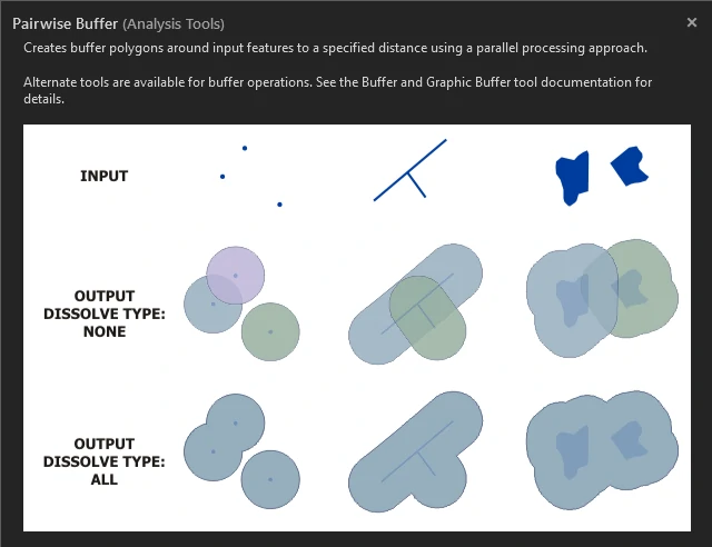
Buffers are polygons that are created around a feature at specified distances. To look for retail site prospects that are within a quarter mile of bike lanes, we’ll first create buffers of existing and proposed bike lanes.

In this part we will use the Pairwise Buffer tool to create a distance of a quarter mile around existing bike lanes. This measurement is a simplified representation of accessibility. Many more factors help define what accessibility means in real terms: mode of transportation, walkability, and road infrastructure.

we apply there parameters to Pairwise Buffer tool:

• Input table = Existing Bike Lanes
• Distance box = 0.25
• Buffer unit box = US Survey Miles
• Method = Planar
• Dissolve Type = Dissolve All Output Features into a Single Feature.

The Dataset

The buffer result

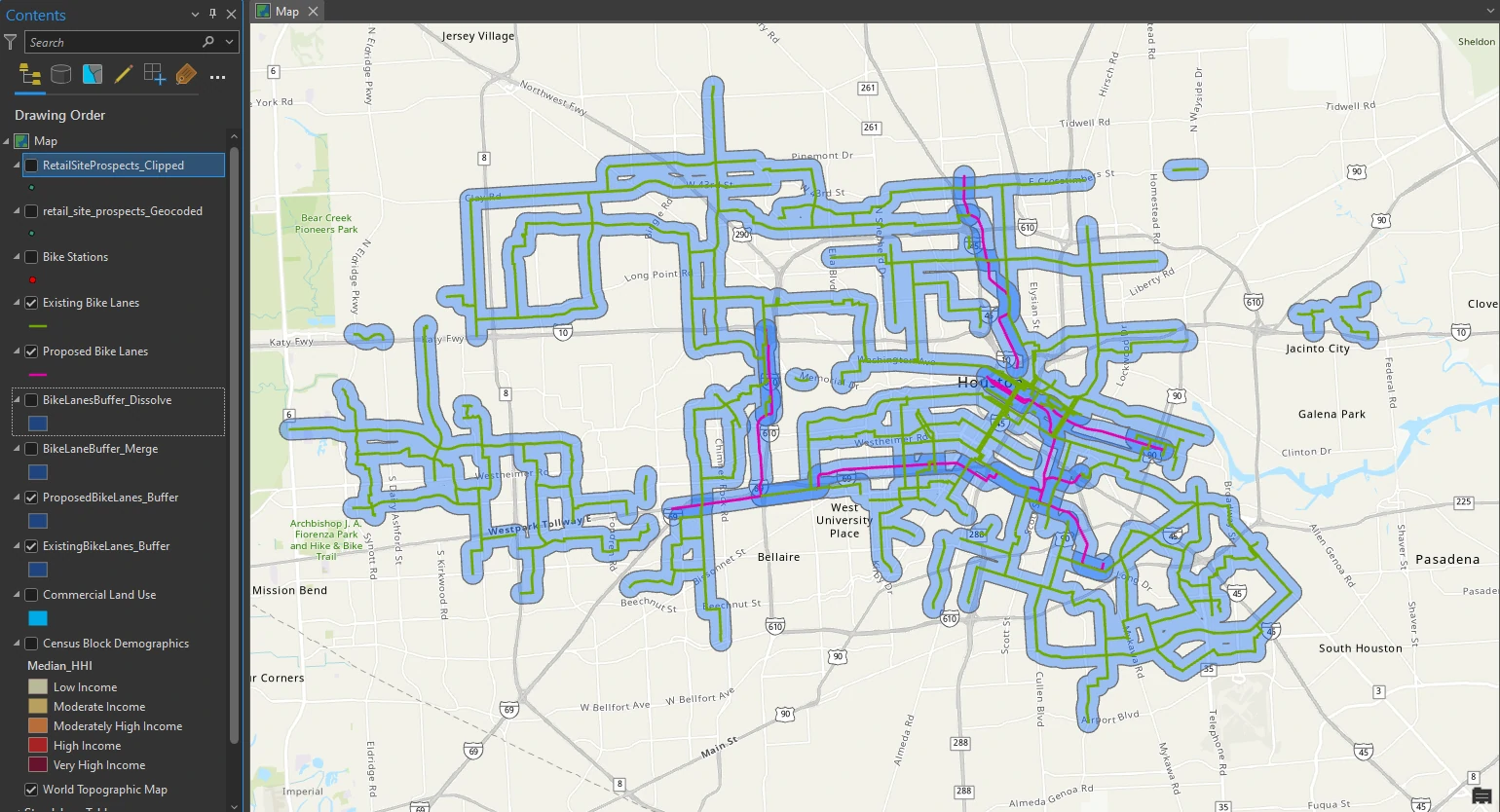
At a glance, we can see a visual cluster of bike lanes in the city of Houston core. We will merge these two buffers together and dissolve them to form one combined buffer.

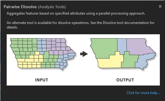
Merge and dissolve features

Currently we have 2 datasets, namely Proposed Bike Lanes and Existing Bike Lanes. To make it easier to analyze, we can merge these datasets and combine them into single dataset by utilize Merge tool and Pairwise Dissolve tool.

Merge tool and Pairwise Dissolve tool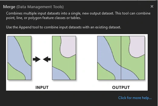

Result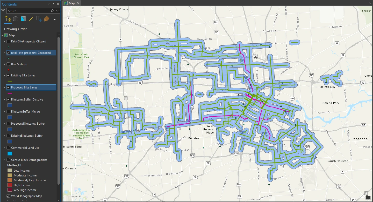

The single buffer layer will now be used as the clip features to extract retail site prospects.

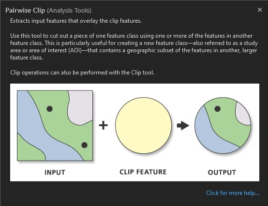
Clip features

Next, we use The Pairwise Clip tool to extracts features using other features as a “cookie cutter” or trim boundary. This tool is particularly useful because we want to find only the retail site features that are within the bike lane buffer, essentially within a quarter mile of an existing or proposed bike lane.

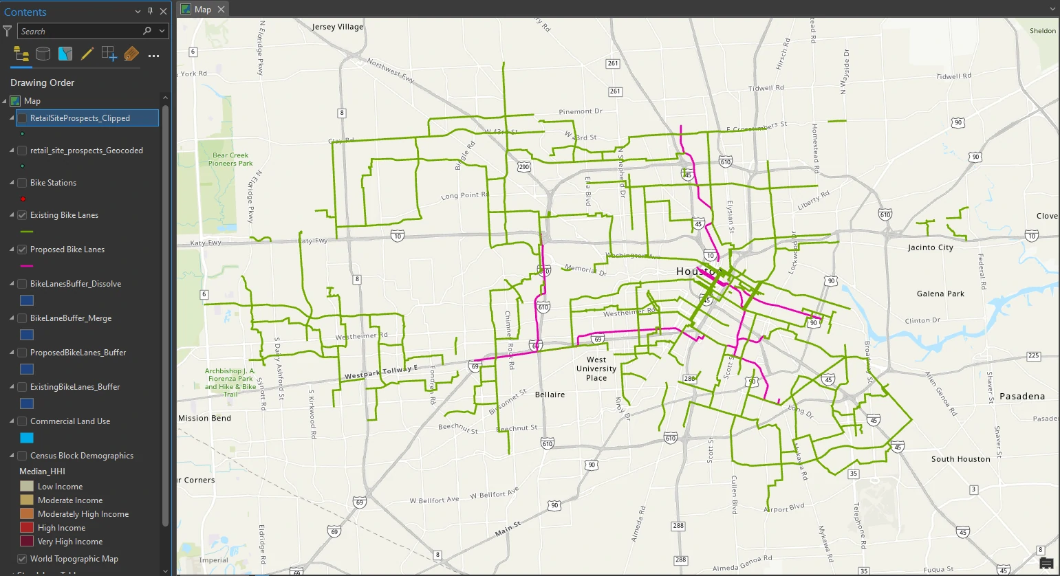
Reviewing this below layer gives we an idea of what we are trying to extract —all the retail site prospects that fall within the boundary of the bike lane buffer. and now only the retail site prospects that are clipped to the bike lanes buffer layer are visible.

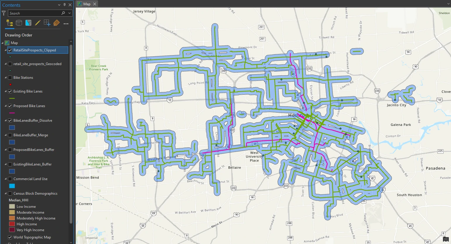
The clip operation reduced the number of retail sites from 28 to 19. We will further reduce the number of retail sites by creating more selections based on additional criteria.

Select by attribute and location

To isolate the census tracts that we have seen throughout this project, we will use the Select By Attributes and Select By Location tools. The Select By Location tool can select features by calculating spatial relationships between layers. This step is also known as a location query.

Current map before selection

The high-end bicycle retail location will require us to look at who the optimal customer is in terms of demographics, based on a profile of our customer’s economic situation. In this project, we will look at moderately high to very high median household income as an ndicator. Customers in these areas may have additional disposable income to spend on high-end bicycles, maintenance, and service.

To do that we will use Select By Attributes and Select By Location tools by using these parameters:

• The expression for Select By Attributes = Where Median_HHI is greater than 63250
• Relationship for Select By Location = Within
• Selecting Features = Census Block Demographics
• Selection Type = Subset from the Current Selection

Selecting a subset from the current selection selects only the retail site prospects that are within the higher median income census block groups. To apply this filter, right-click at the layer, go to Selection, and click Make Layer from Selected Features.

The result after selection

The result of this selection criteria have narrowed the list to just seven retail site prospects.

Create a spatial join

Up to this point, we have used several criteria to narrow the remaining retail site prospects. We will continue to evaluate using additional criteria.

The Bike Stations layer represents shared bikes that members of the community can rent for short rides. Combined with the bike lanes, the placement of bike stations also represents corridors of active cycling infrastructure and offers good visibility for a retail site. We will create a buffer around our final selection of retail site prospects and then perform a spatial join to include attributes of nearby bike stations.

Again we will use Pairwise Buffer tool with these parameters:

• Distance [value or field] = 1
• Buffer unit box = US Survey Miles
• Method = Planar
• Dissolve Type = No Dissolve

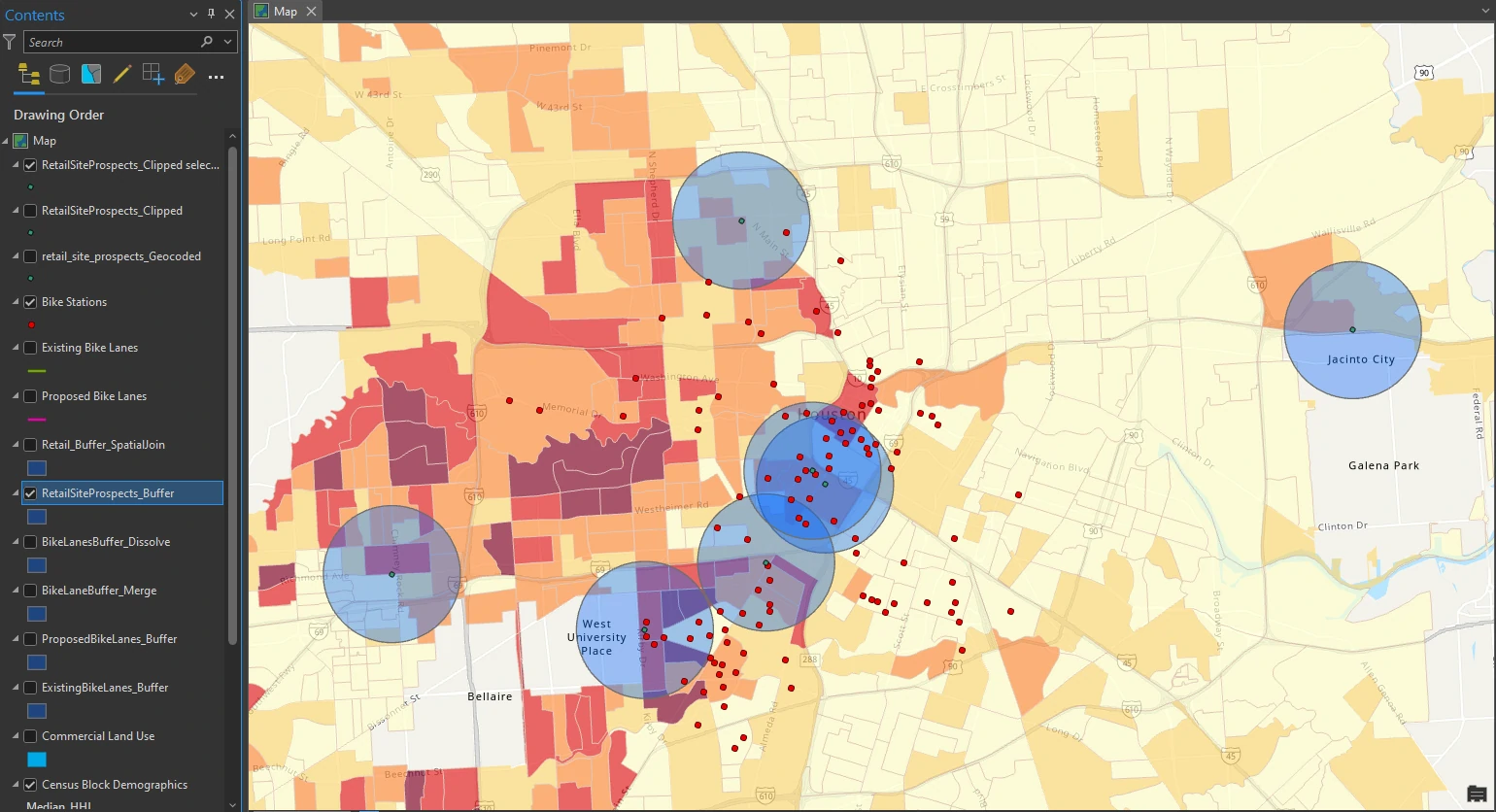
Next, we use Spatial Join to join all parameters within buffer area. we will apply this parameters:

• Target Features = RetailSiteProspects_Buffer
• Join Features = Bike Stations
• Match Option = Intersect

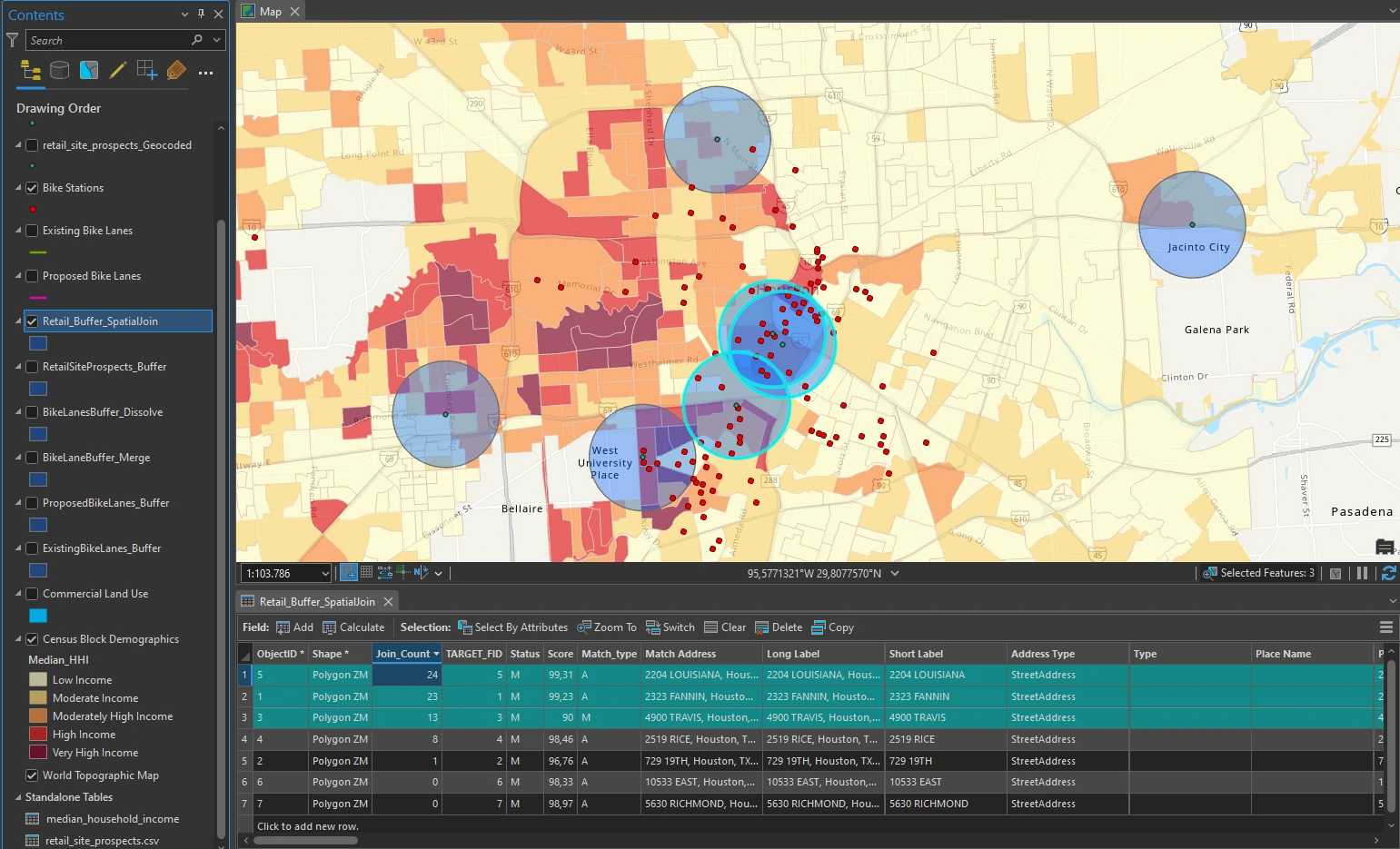
The result of this is a layer with Join_Count attribute that counts all the bike stations in the one-mile buffer around each retail site prospect. We can select the top three rows to highlight them on the map as shown in image below. Or we can use Definition Query to create filter such as Where Join_Count is greater cthan or equal to 13.

Two sites have more than 20 stations around them, and the third site has 13 stations around it. These are good locations based on the amount of infrastructure in the area. Take note of the address of each location.

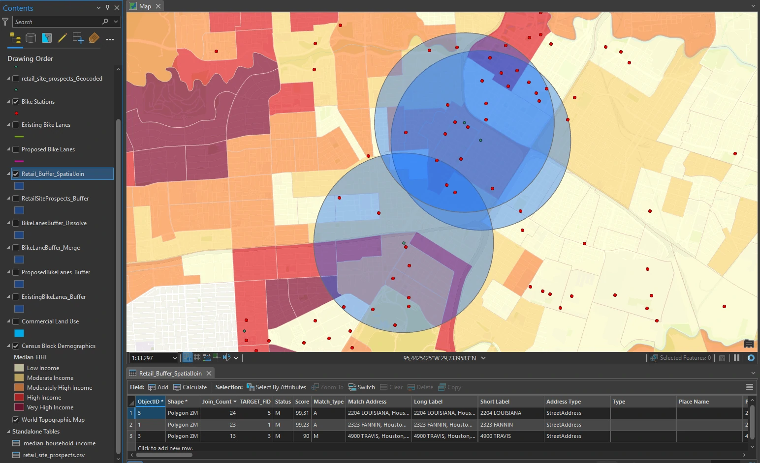
The remaining three retail site prospects are in a great location in the city core, in proximity to bike lanes and multiple bike stations, and in high median household income areas.

Conclusion

Finally, we will look at a few other attributes that may help us decide which site is the most suitable. We maybe need to consider accessibility ratings for walking, transit, and biking and the square footage and cost of each retail site.

Accessibility ratings provide an index for the public to know how accessible a location is. Ratings higher than 80 provide a particularly good indicator of access. In this scenario, a bike rating higher than 80 means that cyclists can access the site easily by bike and can conduct their daily activities by bike.

In this project, cost and square footage are provided and simplified. Often, how much a location costs to purchase or rent could be the main decision factor.

When comparing all three sites, the 4900 Travis St. site has the most square footage and has the lowest cost per square foot. It also has the best biking rating (83), but the lowest transit rating (66). The other retail sites have a slightly higher walking rating. As we can see, detailed information like this can factor into the decision-making process. In this scenario, all three sites are suitable candidates and worthy of consideration.