Species Distribution Modeling (SDMs) with Machine Learning
geospatial
map
distribution models
Introduction
Understanding Species Distribution Models (SDMs)
Where do species thrive, and what environmental conditions make their habitats suitable? These are fundamental questions in ecology, conservation, and land management. Species Distribution Models (SDMs) help answer them by analyzing the relationships between species occurrences and environmental factors to predict where species are most likely (distribution) to be found—both now and in the future.
SDMs are invaluable tools for:
- Ecologists tracking biodiversity changes.
- Agricultural scientists predicting pest outbreaks.
- Conservation biologists identifying priority areas for habitat protection.
- Land-use planners ensuring sustainable development that minimizes ecological impact.
With the growing availability of high-resolution geospatial and climate data, SDMs have become more powerful and accessible than ever—especially with machine learning techniques that enhance prediction accuracy. This page explores a practical SDM workflow using Python and Scikit-Learn, demonstrating how data-driven modeling can map species suitability across landscapes and inform environmental decision-making.
How SDMs Work: Linking Species to Their Environment
At the core of SDMs is a simple yet powerful idea:
Species distributions are shaped by environmental conditions.
By analyzing where a species has been observed and linking those locations to climate, land cover, and other ecological variables, we can model the species’ environmental preferences. This allows us to:
- Identify suitable habitats for species based on existing data.
- Predict new locations where the species might thrive.
- Forecast changes in species distributions under different climate scenarios.
Key Steps in an SDM Workflow
- Conceptualization – Define the research question and species of interest.
- Data Pre-processing – Collect and clean occurrence records and environmental data.
- Model Training & Assessment – Use machine learning (e.g., Scikit-Learn classifiers) to establish species-environment relationships.
- Interpolate & Extrapolate – Apply the model to predict species distribution across space and time.
- Iteration – Refine the model based on new data or improved techniques.
Interpolation vs. Extrapolation: Mapping Species Distributions
Once an SDM is trained, it can be used in two main ways:
-
Interpolation: Mapping species suitability within the same geographic area and environmental conditions used to train the model. This helps identify potential habitats based on known environmental relationships.
-
Extrapolation: Applying the model to new areas or future climate scenarios. This is crucial for predicting how species distributions might shift due to climate change, habitat loss, or human interventions.
By utilizing machine learning, SDMs can process large datasets efficiently and generate highly accurate habitat suitability maps, making them essential tools for modern conservation and ecological research.
Why This Matters
- Biodiversity Conservation – Helps identify critical habitats and inform conservation planning.
- Climate Change Adaptation – Predicts how species might shift in response to changing temperatures and precipitation.
- Invasive Species Management – Identifies areas vulnerable to the spread of non-native species.
- Agriculture & Pest Control – Anticipates crop pest distributions under different environmental conditions.
Whether you’re an ecologist, a data scientist, or just an enthusiast in geospatial sciences, understanding SDMs opens doors to data-driven insights into species-environment interactions.
Data Preparation
Load dataset
We first need to download a geodatabase (here we use a .shp file) denoting presence/absence coordinates, which can be directly loaded into Python as a GeoPandas GeoDataFrame. Here, the CLASS column is a binary indication of the presence/absence of the species. For this project, we are using Joshua trees (Yucca brevifolia) as the example species:
Beside of presence species data, in this project we will train our machine learning classifiers and make spatial predictions of the species distribution over current conditions (1970-2000).
First, we load 19 bioclimatic features (here we use 2.5 arc-minute resolution) from the publicly available WorldClim database (v. 2.1, Fick & Hijmans, 2017).
# Presence data
pa = gpd.GeoDataFrame.from_file("../data/jtree.shp")

#Raster data
for f in sorted(glob.glob('data/bioclim/bclim*.asc')):
    shutil.copy(f,'inputs/')
raster_features = sorted(glob.glob('inputs/bclim*.asc'))
print('\nThere are', len(raster_features), 'raster features.')
There are 19 raster features.
Presence Species Data
We can map the species presences (pa==1). 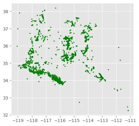
Background Data
We can map the background points (pa == 0). 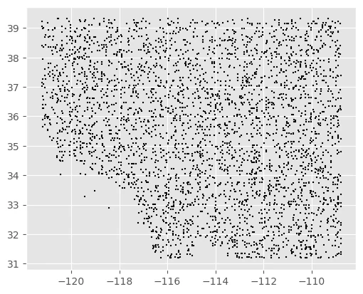
Preparing Raster Data into Machine Learning
By using pyimpute library, we generate the raster maps of suitability into more acceptable data input for Machine learning model.
train_xs, train_y = load_training_vector(pa, raster_features, response_field='CLASS')
target_xs, raster_info = load_targets(raster_features)
train_xs.shape, train_y.shape
Model
In this project we used some models that will learn from our dataset and raster data and try to predict the outcome value. the models are:
- Random Forest
- Extra Tree
- Xgboost
- Light gradien boosting model (lgbm)
Initiate Models
By using model_pred.model_collection we can initiate all models yang we want to use for this prediction. This function will return default condition for all models and we need to change some parameters inside this function to get more accurate and robust models.
list_model = ['random_forest','extra_tree',"xgb","lgbm"]
result = model_pred.model_collection(list_model,types='classification')
result
This function requires the following parameters:
- list_model (
list): list of models - types (
string): type of machine learning that we handle
[['random_forest', RandomForestClassifier()],
 ['xgb',
  XGBClassifier(base_score=None, booster=None, callbacks=None,
                colsample_bylevel=None, colsample_bynode=None,
                colsample_bytree=None, device=None, early_stopping_rounds=None,
                enable_categorical=False, eval_metric='logloss',
                feature_types=None, gamma=None, grow_policy=None,
                importance_type=None, interaction_constraints=None,
                learning_rate=None, max_bin=None, max_cat_threshold=None,
                max_cat_to_onehot=None, max_delta_step=None, max_depth=None,
                max_leaves=None, min_child_weight=None, missing=nan,
                monotone_constraints=None, multi_strategy=None, n_estimators=None,
                n_jobs=None, num_parallel_tree=None, random_state=None, ...)],
 ['extra_tree', ExtraTreesClassifier()],
 ['lgbm', LGBMClassifier(device_type='gpu', n_jobs=-1)]]
Cross Validation Training
To obtain a more precise and robust model, we can perform cross-validation on our data and calculate various metrics to evaluate how well the model, with its default hyperparameters, learns from the dataset. By using model_pred.cv_model_train we can create cross validation process for some models that we initiate previously.
result,proba = model_pred.cv_model_train(train_x, train_y,
                    list_model=list_model,types='classification',n_splits=5)
This function requires the following parameters:
- train_xs (
dataframe): independent dataframe - train_ys (
dataframe): dependent dataframe - list_model (
list): list of models - types (
string): type of machine learning that we handle - n_splits (
int): numebr of split in cross validation
Finished training for model:
random_forest
xgb
extra_tree
All models exhibit nearly identical values across all metrics, with differences on the order of $10^{−3}$, particularly in the standard deviation of the accuracy metric, which is also on the order of $10^{−3}$. This indicates a high level of stability in the model training process.
| Method | accuracy | accuracy_std | balanced_acc | balanced_acc_std | F1 | F1_std | AUC | AUC_std | AUC_ROC | AUC_ROC_std | Recall | Recall_std | Precision | Precision_std | Fit Time | Pred Time | |
|---|---|---|---|---|---|---|---|---|---|---|---|---|---|---|---|---|---|
| 0 | random_forest | 0.9364 | 0.0067 | 0.9351 | 0.0073 | 0.9363 | 0.0067 | 0.9863 | 0.0034 | 0.984 | 0.0036 | 0.9511 | 0.0045 | 0.9325 | 0.012 | 0.5186 | 0.0152 |
| 1 | lgbm | 0.9365 | 0.0054 | 0.9347 | 0.0053 | 0.9364 | 0.0054 | 0.982 | 0.0062 | 0.981 | 0.0047 | 0.9575 | 0.0075 | 0.9272 | 0.0044 | 0.6605 | 0.007 |
| 2 | extra_tree | 0.9365 | 0.0032 | 0.9354 | 0.0032 | 0.9365 | 0.0032 | 0.9818 | 0.0013 | 0.9765 | 0.0019 | 0.9498 | 0.0065 | 0.9337 | 0.0042 | 0.2104 | 0.0154 |
| 3 | xgb | 0.9326 | 0.0023 | 0.9309 | 0.0025 | 0.9325 | 0.0023 | 0.9817 | 0.0021 | 0.9802 | 0.0025 | 0.9531 | 0.0044 | 0.9244 | 0.0055 | 0.2874 | 0.0068 |
Training Model
After examining cross validation training result, we can move to training our data by calling model_pred.modeling function. This function will return its model, its prediction and probability, its prediction and time duration.
models,models_calib,names_model,probs_model,probs_true_model,probs_dual_model,probs_bool_model,pred_model,time_1,time_2 = model_pred.modeling(
   X_train=train_xs,X_test=target_xs,y_train=train_y,y_test=None ,list_model=list_model,
   types='classification',tresh=0.5,detail=False, method='isotonic')
This function requires the following parameters:
- train_xs (
dataframe): independent train dataframe - train_ys (
dataframe): dependent train dataframe - target_xs (
dataframe): independent test dataframe - test_ys (
dataframe): dependent test dataframe - list_model (
list): list of models - types (
string): type of machine learning that we handle - tresh (
int): numebr of threshold to seperate 2 class - detail (
boolean): generate plot after training - method (
string): method to calibrate our training
we have done with these models:
Random Forest
Xgboost
Extra Tree
lightgbm
Generate Spatial Prediction After Training
After training, we can make a prediction using all of the dataset and safe it in raster format. We have a responses.tif raster which is the predicted class (0 or 1) and probability_1.tif with a continuous suitability scale.
if not os.path.exists('outputs'):
        os.makedirs('outputs')
for idx, model in enumerate(models):
        model.fit(train_xs, train_y)
        os.mkdir('outputs/' + names_model[idx] + '-images')
        impute(target_xs, model, raster_info, outdir='outputs/' + names_model[idx] + '-images',
                class_prob=True, certainty=True)
Aggregate All Prediction
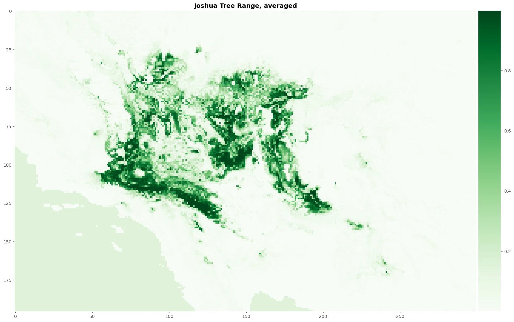
Let’s average the continuous output for the four models and plot our map. This process will help use to create normalize prediction value to get more robust result and create plot image to see the result.
distr_rf = rasterio.open("outputs/Random Forest Classifier-images/probability_1.0.tif").read(1)
distr_et = rasterio.open("outputs/Extra Tree-images/probability_1.0.tif").read(1)
distr_xgb =  rasterio.open("outputs/Xgboost-images/probability_1.tif").read(1)
distr_lgbm =  rasterio.open("outputs/lightgbm-images/probability_1.0.tif").read(1)
distr_averaged = (distr_rf + distr_et + distr_xgb + distr_lgbm)/4
fig, axes = plt.subplots(1, 1, figsize=(20, 15))
im = axes.imshow(distr_averaged, cmap="Greens", interpolation='nearest')
axes.grid()
axes.set_title('Joshua Tree Range, averaged', fontweight = 'bold')
divider = make_axes_locatable(axes)
cax = divider.append_axes('right', size='5%', pad=0.05)
fig.colorbar(im, cax=cax, orientation='vertical')
plt.show()
The result
Images above will help use to predicting a mapping species suitability within the same geographic area and environmental conditions. SDMs help us to analyzing and predicting the relationships between species occurrences and environmental factors to predict where species are most likely (distribution) to be found—both now and in the future.
Source
- https://daniel-furman.github.io/Python-species-distribution-modeling/