Species Distribution Modeling using Maxent Model

geospatial

map

spatial optimization

maxent model

Introduction

Understanding Species Distribution Models (SDMs)

Maxent is a species distribution modeling (SDM) system that uses species observations and environmental data to predict where a species might be found under past, present or future environmental conditions.

It’s a presence/background model. Maxent uses data on where a species is present and, instead of data on where it is absent, it uses a random sample of the landscape where you might expect to find that species. This is convenient because it reduces data collection requirements, but it also introduces some unique challenges for fitting and interpreting models.

Formally, Maxent estimates habitat suitability (i.e. the fundamental niche) using:

• species occurrence records (y = 1),
• randomly sampled “background” location records (y = 0), and
• environmental covariate data (x) for each location of y.

Maxent doesn’t directly estimate relationships between presence/background data and environmental covariates (so, not just y ~ x). Instead, it fits a series of feature transformatons to the covariate data (z = f(x)), like computing quadratic transformations or computing the pairwise products of each covariate.

Maxent then estimates the conditional probability of finding a species given a set of environmental conditions as:

This can be interpreted as: “the relative likelihood of observing a species at any point on the landscape is determined by differences in the distributions of environmental conditions where a species is found relative to the distributions at a random sample across the landscape.”

A null model would posit that a species is likely to be distributed uniformly across a landscape; you’re equally likely to find it wherever you go. Maxent uses this null model—the “background” conditions—as a prior probability distribution to estimate relative suitability based on the conditions where species have been observed.

Because of this formulation, the definition of both the landscape and the background are directly related to the definition of how habitat suitability is estimated. These should be defined with care.

in this project, We’ll use this model for extracting raster data from points and polygons, assigning sample weights based on sample density, and creating spatially-explicit train/test data, while also showing general patterns

Data Preparation

Load dataset

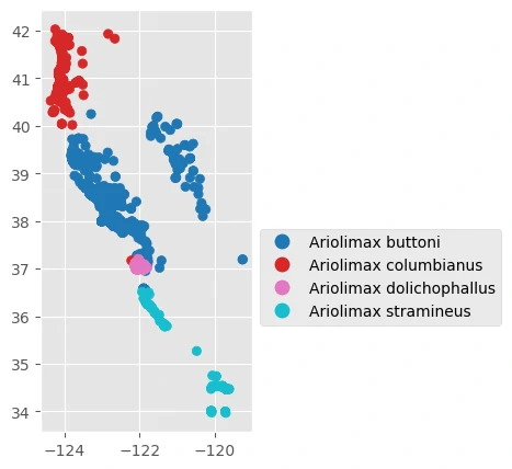
The sample data we’ll use includes species occurrence records from the genus Ariolimax, a group of North American terrestrial slugs, as well as some climate and vegetation data.

Raster Data

Environmental data are typically provided as image data with coordinate reference information, or “raster data”. We load raster data that contains some parameters, there are:

• Cloud Cover Mean
• Cloud Cover Stdv
• LAI Mean (vegetation growth)
• LAIS tdv vegetation growth
• Surface Temp Mean
• Surface Temp Stdv

path = os.getcwd()+'/data'
raster_names = [
    "ca-cloudcover-mean.tif",
    "ca-cloudcover-stdv.tif",
    "ca-leafareaindex-mean.tif",
    "ca-leafareaindex-stdv.tif",
    "ca-surfacetemp-mean.tif",
    "ca-surfacetemp-stdv.tif",
]
rasters = [f"{path}/{raster}" for raster in raster_names]
labels = ["CloudCoverMean", "CloudCoverStdv", "LAIMean", "LAIStdv", "SurfaceTempMean", "SurfaceTempStdv"]

Point-Format Data

Occurrence data are typically recorded with latitude/longitude coordinates for a single location, also known as “point-format data”. We load point-format that contains locations on the landscape where a species has been observed and identified and recorded as present in an x/y location.

We then model the relative likelihood of observing that species in other locations based on the environmental conditions where that species is observed.

gdf = gpd.read_file(os.getcwd()+'/data/ariolimax-ca.gpkg')

Next, we can plot data from four species of Banana Slug across California.

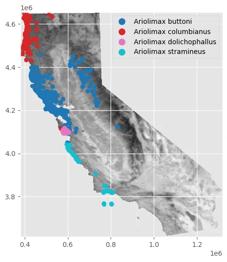
And we can add raster data into our previous plot to get comparison between this two data.

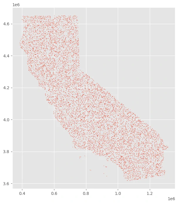
Drawing random pseudoabsence locations

In addition to species occurrence records (where y = 1), species distributions models often require a set of random pseudo-absence/background points (y = 0). These are a random geographic sampling of where you might expect to find a species across the target landscape.

The background point distribution is extremely important for presence-only models, and should be selected with care.

By using maps.random_sempling we can generate random pseudoabsence as background data. This process can be calculate by raster and/or point-format data as well.

pseudoabsence = maps.random_sampling(main_data_raster, count=10000, 
                                    types= 'spatial', markersize=0.25,
                                    ignore_mask=False, main_data=None,figsize=(8,8))

This function requires the following parameters:

• main_data_raster (raster data): raster data
• count (int): number of pseudoabsence point
• types (string): type of pseudoabsence [spatial, bias]
• markersize (int): size of marker on plot
• ignore_mask (boolean): to use the rectangular bounds of the raster to draw samples
• main_data (geodataframe): point-format data
• figsize (tuple): size of figure

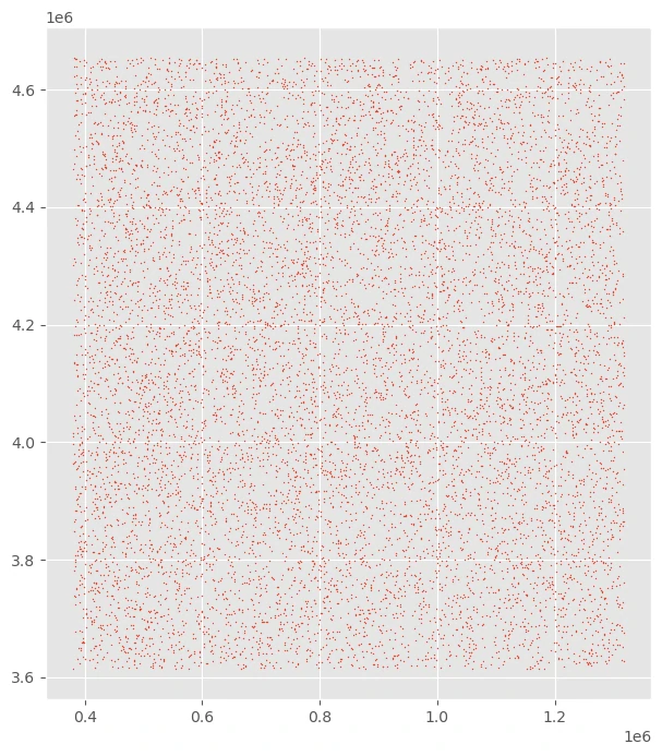
uniform random geographic sample from unmasked locations within a raster’s extent

we can use raster data to create a uniform random geographic sample from unmasked locations within a raster’s extent.

uniform random geographic sample from unmasked locations within a raster’s extent

we can use raster data to use the rectangular bounds of the raster to draw samples.

From a bias raster

We could also provide a “bias” file, where the raster grid cells contain information on the probability of sampling an area. Bias adjustments are recommended because species occurrence records are often biased towards certain locations (near roads, parks, or trails).

The grid cells can be an arbitrary range of values. What’s important is that the values encode a linear range of numbers that are higher where you’re more likely to draw a sample. The probability of drawing a sample is dependent on two factors: the range of values provided and the frequency of values across the dataset.

We’ll use the leaf area index (LAI) covariate to select more background samples from highly vegetated areas.

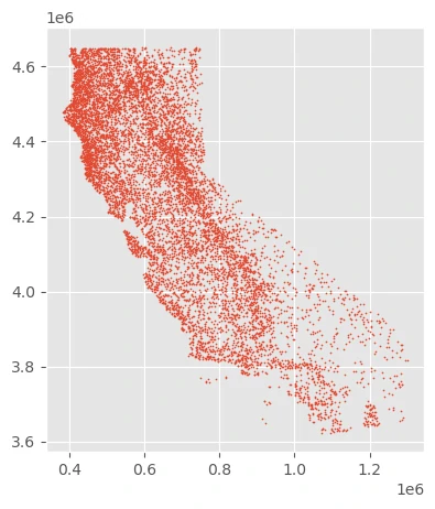
We can see that we are selecting a disproportionately high number of points along California’s coast - home to dense redwood forests where slugs thrive - and disproportionately few samples in the dry deserts in the southeast.

From a vector polygon

Another way to address bias would be to only select points inside area where that species is known to occur (within a certain ecoregion, for example).

The Ariolimax dataset contains occurrence records for four species within the genus. If we’re interested in understanding the distributions of only one of them, we could construct a rudimentary “range map” for this genus by computing the bounding geometry of all points then sampling within those bounds.

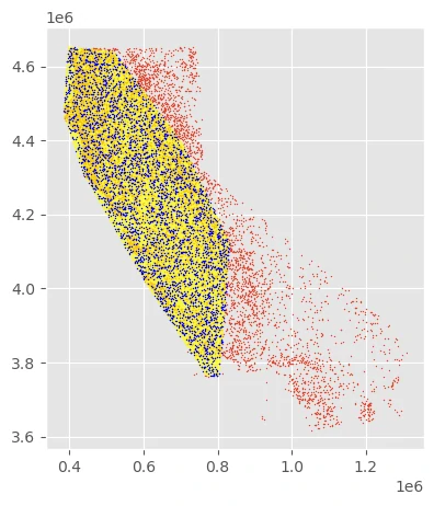
• The yellow polygon above shows the simple “range map”.
• The blue points are point samples selected from within that range.
• The red points are the uniform sample, plotted for reference.

Point annotation

Annotation refers to extracting raster values at the each point occurrence record and storing those records together in a GeoDataFrame. Once you have your presence and pseudo-absence records, you can annotate these records with the corresponding covariate data.

It also allows you to pass multiple raster files, which can be in different projections, extents, or grid sizes. This means you don’t have to explicitly re-sample your raster data prior to analysis, which is always a chore.

presence, background, zs = generate_raster_df(main_data, background_bias,
                                        main_data_raster, area_hull=None, labels=[], figsize=(6,9), row_col=[2,3])

This function requires the following parameters:

• main_data (geodataframe): point-format data
• main_data_raster (raster data): raster data
• background_bias (geodataframe): point-format from background
• area_hull (geodataframe): geometry area
• labels (list): label of raster data
• row_col (list): coordinate of subplot
• figsize (tuple): size of figure

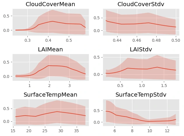
Next let’s plot some histograms to understand the similarities and differences between the conditions at presence locations and at background locations.

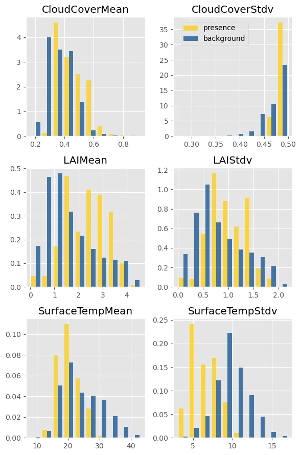
This checks out. Slugs are commonly found in areas with higher annual cloud cover, consistently cool temperatures, and high vegetation growth (even after adjusting for bias and oversampling areas with high LAI).

Zonal statistics

This code reads an array of raster data covering the extent of a polygon, masks the areas outside the polygon, and computes summary statistics such as the mean, standard deviation, and mode of the array.

Geographic sample weights

This step help us to handle geographic information during model selection or in model scoring.

Add spatial information to a model is to compute geographically-explicit sample weights. elapid does this by calculating weights based on the distance to the nearest neighbor. Points nearby other points receive lower weight scores; far-away points receive higher weight scores.

presence, background = sample_weight(main_data, background_bias, 
                                    n_neighbors=1, types='distance')

This function requires the following parameters:

• main_data (geodataframe): point-format data
• background_bias (geodataframe): point-format from background
• n_neighbors (int): number of neighbors that will be considering for weight.
• types (list): type of sample weight [density, distance]

Compute weights based on the distance to the nearest point

This code with distance will calculate weights based on the distance to the nearest neighbor.

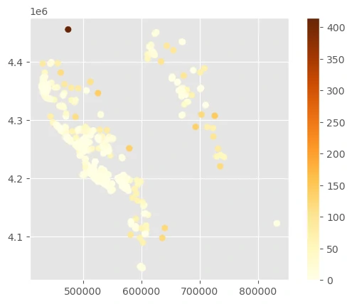
There’s one lone point in the northwest corner that is assigned a very high weight because it’s so isolated.

Compute weights based on the distance to the nearest point

This code with density will compute the average distance from each point to all other points, computing sample weights from point density instead of the distance to the single nearest point. This may be useful if you have small clusters of a few points far away from large, densely populated regions.

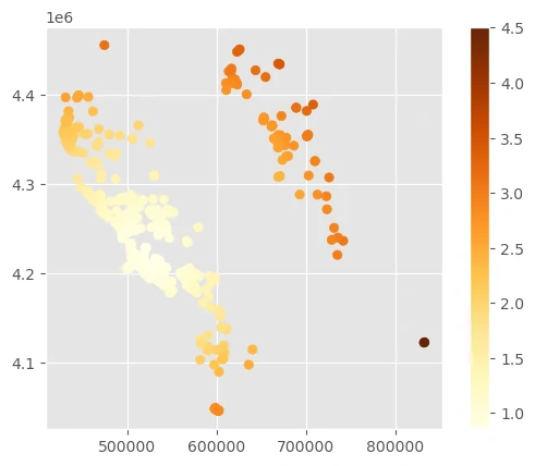
As you can see, there are tradeoffs for finding the best sample weights depending on the spatial distributions of each occurrence dataset. We’ll use the sample density weights here to upweight the samples in the sierras (the northeastern cluster of points).

Train / test splits

Uniformly random train/test splits are generally discouraged in spatial modeling because of the strong spatial structure inherent in many datasets. The non-independence of these data is referred to as spatial autocorrelation. Using distance- or density-based sample weights is one way to mitigate these effects. Another is to split the data into geographically distinct train/test regions to try and prioritize model generalization.

xtrain, ytrain, sample_weight_train, xtest, ytest, sample_weight_test = maps.data_prep(main_data, background_bias, target_col='', weight_col='', 
                    types= 'checkerboard', grid_size=50000, 
                    fold=0, n_splits=3, training=True)

This function requires the following parameters:

• main_data (geodataframe): point-format data
• background_bias (geodataframe): point-format from background
• target_col (string): targeted column name (dependent variable)

• weight_col (string): sample weight column name

• grid_size (string): grid size to split train and test dataset
• fold (string): number of fold in cross validation
• n_splits (string): number splits in cross validation
• training (boolean): is do training

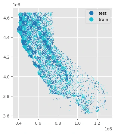
Checkerboard splits

With a “checkerbox” train/test split, points are intersected along a regular grid, and every other grid is used to split the data into train/test sets.

The height and width of the grid used to split the data is controlled by the grid_size parameter. This should specify distance in the units of the point data’s CRS.

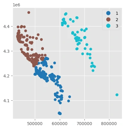
Geographic k-fold splits

Create k geographically-clustered folds using the GeographicKFold cross validation strategy. This method is effective for understanding how well models fit in one region will generalize to areas outside the training domain.

This method uses KMeans clusters fit with the x/y locations of the point data, grouping points into spatially distinct groups. This cross-validation strategy is a good way to test how well models generalize outside of their training extents into novel geographic regions.

Modeling

Fitting models using default settings, then evaluate the effects of different forms of train/test splitting strategies.

Initiate Models

By using model_pred.model_collection we can initiate all models yang we want to use for this prediction. This function will return default condition for all models and we need to change some parameters inside this function to get more accurate and robust models.

list_model = ['random_forest','extra_tree',"xgb","lgbm"]
result = model_pred.model_collection(list_model,types='classification')
result

This function requires the following parameters:

• list_model (list): list of models
• types (string): type of machine learning that we handle

[['maxent_model', MaxentModel()]]

Training Model

After examining cross validation training result, we can move to training our data by calling model_pred.modeling function. This function will return its model, its prediction and probability, its prediction and time duration.

models,models_calib,names_model,probs_model,probs_true_model,probs_dual_model,probs_bool_model,pred_model,time_1,time_2 = model_pred.modeling(
   X_train=train_xs,X_test=target_xs,y_train=train_y,y_test=None ,list_model=list_model,
   types='classification',tresh=0.5,detail=False, method='isotonic')

This function requires the following parameters:

• train_xs (dataframe): independent train dataframe
• train_ys (dataframe): dependent train dataframe
• target_xs (dataframe): independent test dataframe
• test_ys (dataframe): dependent test dataframe
• list_model (list): list of models
• types (string): type of machine learning that we handle
• tresh (int): numebr of threshold to seperate 2 class
• detail (boolean): generate plot after training
• method (string): method to calibrate our training

we have done with these models:
Maxent Model

Evaluate the model

After training our data, we can evaluate the model to determine how well our model is during learning process. by calling model_pred.modeling function. This function will return its model, its prediction and probability, its prediction and time duration.

print_score(y_test,y_pred,y_probs=None,types='classification',labels=None,time1=1,
            time2=2,X_train=None,y_train=None,y_pred_test=None,X_test=None,
            axis_labels=['Actual','Predicted'],cost_mat=None,sample_weight=None)

This function requires the following parameters:

• y_test (dataframe): y test dataframe
• y_pred (dataframe): y prediction dataframe from model
• types (string): type of machine learning that we handle
• labels (list): label to shown in graph
• time1 (time): time when start modeling
• time2 (time): time when end modeling
• X_train (dataframe): X train dataframe
• y_train (dataframe): y train dataframe
• y_pred_test (dataframe): y prediction dataframe from test dataset
• X_test (dataframe): X test dataframe
• axis_labels (list): label to shown in graph
• cost_mat (list): list of cost per each error
• sample_weight (list): sample weight for test and training process

confusion matrix = 
[[2169   99]
 [ 277  611]]

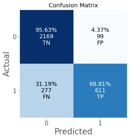
accuracy_score =  0.8809
balanced_accuracy_score =  0.8222
Logloss =  0.4926
Brier score loss (the smaller the better) =  0.0954

homogeneity score =  0.3864
completeness score =  0.4306
v measure score =  0.4073
adjusted rand score =  0.5544
adjusted mutual info score =  0.4071

precision score =  0.8606
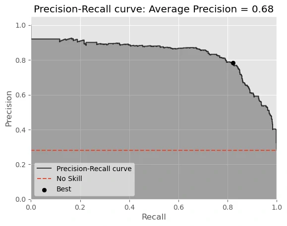
average precision score =  0.6799
recall score =  0.6881

F1 score =  0.7647
F2 score =  0.7168
F3 score =  0.7021
F_beta score (0.5) =  0.8195

AUC of Precision-Recall Curve on Testing =  0.8347
Best Threshold for Precision-Recall Curve = 0.292900
F-Score = 0.802
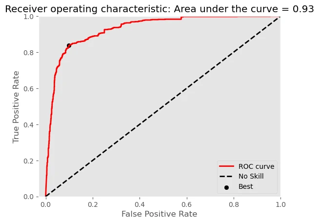
AUC of ROC =  0.9304

Best Threshold for ROC = 0.247900
G-Mean = 0.869
Best Threshold with Youden’s J statistic = 0.247900

Cohens kappa =  0.6863
Gini =  0.6694

Expected Approval Rate =  0.225
Expected Default Rate =  0.1394

classification_report
              precision    recall  f1-score   support

           0       0.89      0.96      0.92      2268
           1       0.86      0.69      0.76       888

    accuracy                           0.88      3156
   macro avg       0.87      0.82      0.84      3156
weighted avg       0.88      0.88      0.88      3156

time span=  0:00:01.383780

As you can see our model has good result, with:

• accuracy_score = 0.8809
• AUC of ROC = 0.9304

but need to mention that our model has low recall score recall score = 0.6881 due to high FN value.

we can used output model to create partial dependence plots (PDP) to show how model predictions vary across the range of covariates

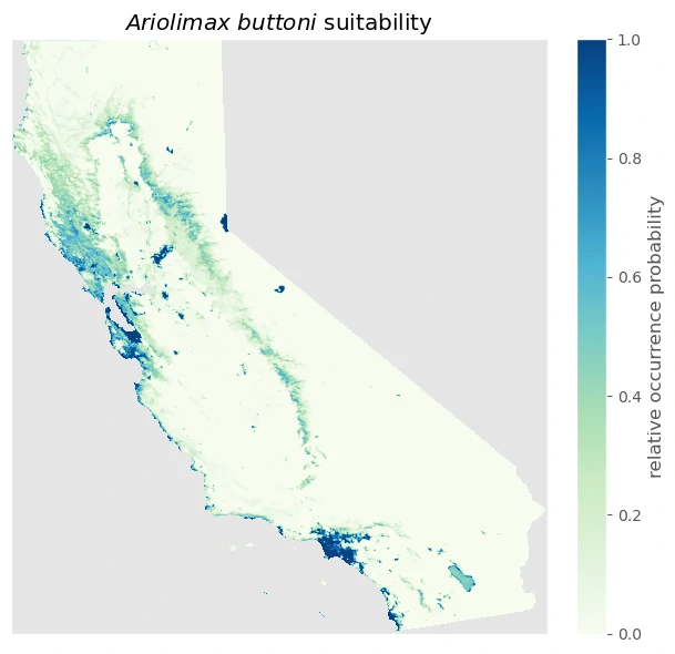
Result

we can plot the suitability predictions

Source

• https://earth-chris.github.io/elapid/sdm/maxent/