Species Distribution Modeling (SDMs) with Unsupervised Learning
geospatial
map
distribution models
Introduction
Modeling Species’ Geographic Distributions: A Case Study of South American Mammals
Understanding where species live and how their habitats are shaped by environmental conditions is a fundamental challenge in conservation biology. By modeling species distributions, scientists can identify critical habitats, assess environmental threats, and predict how species might respond to climate change or habitat destruction.
In this project, we explore how machine learning can be applied to model the geographic distribution of two South American mammals. Using past species occurrence data and 14 environmental variables, we train a model to estimate their suitable habitats. Since we only have positive observations (where the species has been found, but no records of where it does not occur), we approach this as a density estimation problem using the Unsupervised Learning.
Why Density Estimation?
Unlike traditional classification problems that distinguish between presence and absence, species distribution modeling often relies on presence-only data. This means we do not have labeled examples of areas where the species is definitively absent — we only know where it has been observed.
To handle this, we use Unsupervised Learning to recognize the patterns of known presence locations and then predicts areas that share similar environmental characteristics—potentially indicating suitable habitat.
Mapping Species Distributions
Once the model is trained, we use it to create a predictive map of species distributions across South America. To make the visualization clearer, we also plot coastlines and national boundaries, providing geographic context for conservation efforts.
This step allows us to:
- Identify key habitats that need protection.
- Understand geographic limitations that may impact species movement.
- Compare species distributions across countries and regions to guide conservation policies.
Why This Study Matters
- Conservation Planning: Helps prioritize areas for habitat protection.
- Climate Change Adaptation: Predicts how species may shift due to global warming.
- Data-Driven Decision Making: Provides insights for researchers, policymakers, and ecologists.
By leveraging machine learning and geospatial analysis, this study demonstrates how advanced modeling techniques can enhance species conservation efforts—ensuring that we protect biodiversity in an era of environmental change.
Data Preparation
The dataset, originally provided by Phillips et al. (2006), includes:
- Species occurrence points (where two species has been observed). The two species are: - Bradypus variegatus, the brown-throated sloth. - Microryzomys minutus, also known as the forest small rice rat, a rodent that lives in Peru, Colombia, Ecuador, Peru, and Venezuela.
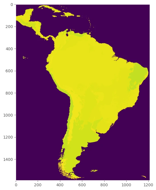
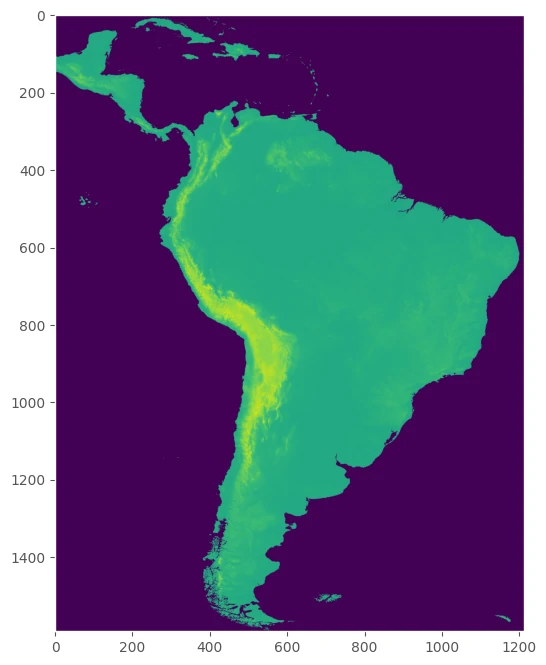
- 14 environmental variables, which may include: - Climate factors (temperature, precipitation, humidity). - Land cover types (forests, grasslands, urban areas). - Elevation and topography (mountainous vs. lowland regions). - Proximity to water bodies (rivers, lakes, coastlines).
By analyzing how these factors correlate with species locations, we can predict areas where the species is likely to exist but has not yet been observed.
Load dataset
The point-format data is easier to load as it stored in csv format. We can utilize pandas or geopandas to load it. Meanwhile, Raster or map grid data is need special process to load them.
We can utilize numpy.fromfile function to read all data in map grid dataset and wrapped it in specific function like below code.
def read_file(fname):
    """Read coverage grid data; returns array of
    shape [n_rows, n_cols]. """
    f = open(fname)
    # Skip header
    for i in range(6):
        f.readline()
    X = np.fromfile(f, dtype=np.float32, sep=" ", count=-1)
    f.close()
    return X.reshape((n_rows, n_cols))

def load_dir(directory):
    """Loads each of the coverage grids and returns a
    tensor of shape [14, n_rows, n_cols].
    """
    data = []
    for fpath in glob("%s/*.asc" % normpath(directory)):
        fname = split(fpath)[-1]
        fname = fname[:fname.index(".")]
        X = read_file(fpath)  #np.loadtxt(fpath, skiprows=6, dtype=np.float32)
        data.append(X)
    return np.array(data, dtype=np.float32)
train = pd.read_csv(r'..\data\sdm sklearn\samples\alltrain.csv')
test = pd.read_csv(r'..\data\sdm sklearn\samples\alltest.csv')
coverages = load_dir(r"..\data\sdm sklearn\coverages")
Point-format dataset
| species | dd long | dd lat | |
|---|---|---|---|
| 0 | microryzomys_minutus | -64.7 | -17.85 |
| 1 | microryzomys_minutus | -67.8333 | -16.3333 |
| 2 | microryzomys_minutus | -67.8833 | -16.3 |
| 3 | microryzomys_minutus | -67.8 | -16.2667 |
| 4 | microryzomys_minutus | -67.9833 | -15.9 |
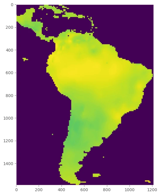
Raster or map grid dataset
Model
Initiate Models
By using maps.sdm_unsupervised_model we can initiate and make model learn from both point-format dataset and map grid dataset. This code by default using One-Class Support Vector Machine as Unsupervised Machine Learning model and we can change it at model_list parameter. To generate fix output from grid map, this code need n_rows_cols, grid_size, left_lower_corner to determine grip map output.
This code will return models, y_test, y_probs, train_pred that we can used for evaluation, generate output for other area.
models, y_test, y_probs, train_pred = maps.sdm_unsupervised_model(main_data_train, main_data_test, coverages, n_rows_cols=[1592,1212], grid_size=0.05, left_lower_corner=[-94.8,-56.05], model_list=['one_class_svm'], name='', is_land= False,is_plot=True, coord_list=[])
This function requires the following parameters:
- main_data_train (
dataframe): point-format dataset - main_data_test (
dataframe): point-format dataset - coverages (
array): collection of grid map in array - n_rows_cols (
list): number of row and columns in grid map - grid_size (
float): grid size of grid map - left_lower_corner (
list): left lower coordinate - model_list (
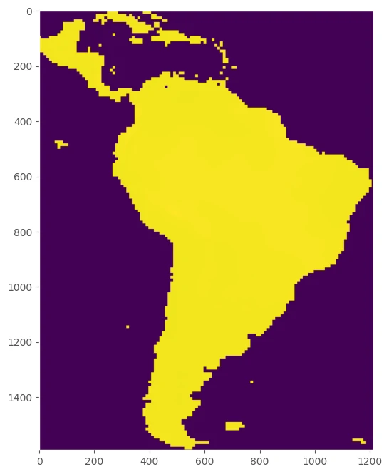
list): list of model name - is_land (
boolean): is need to only select land area - is_plot (
boolean): is need to generate plot - coord_list (
list): coordinate columns name
Evaluation
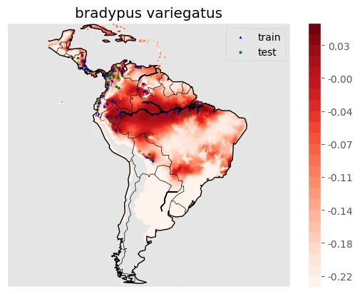
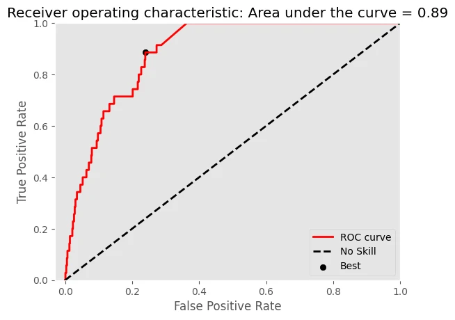
- bradypus variegatus
-Logloss = 0.1008
-AUC of ROC = 0.8859
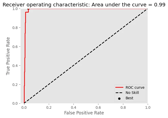
- microryzomys minutus
-Logloss = 0.0907
-AUC of ROC = 0.9934
The result
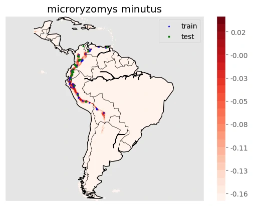
Images above will help use to predicting a mapping species suitability within the same geographic area and environmental conditions. SDMs help us to analyzing and predicting the relationships between species occurrences and environmental factors to predict where species are most likely (distribution) to be found—both now and in the future.
Source
- “Maximum entropy modeling of species geographic distributions” S. J. Phillips, R. P. Anderson, R. E. Schapire - Ecological Modelling, 190:231-259, 2006.