Recommendation System 101
Recommendation
Optimization
matchmaking
- Recommendation System 101
What is recommender systems?
Systems that could predict what an individual user liked and mirror related items to the user in highly visible sections of the web or apps.
Recommender systems draw on both machine learning and data mining techniques. But, machine learning models are more typical because user preferences develop over time and data mining is less conducive to solving tasks with a limited amount of data. Machine learning, though, can be used to make inferences and gradually learn from user behavior and optimize recommendations through extensive trial and error.
The Prediction Problem
Given a matrix of m users and n items. Each row of the matrix represents a user and each column represents an item. The value of the cell in the i th row and the j th column denotes the rating given by user i to item j. This value is usually denoted as r_ij.
In this approach, aims to predict these missing values (from that matrix) using all the information it has at its disposal (the ratings recorded, data on movies, data on users, and so on). If it is able to predict the missing values accurately, it will be able to give great recommendations.
The ranking problem
Ranking is the more intuitive formulation of the recommendation problem. Given a set of n items, the ranking problem tries to discern the top k items to recommend to a particular user, utilizing all of the information at its disposal.
It is easy to see that the prediction problem often boils down to the ranking problem. If we are able to predict missing values, we can extract the top values and display them as our results.
The long tail problem
The whole point of recommender systems is to surface items in what we call “the long tail.” Imagine this is a plot of the sales of items of every item in our catalog, sorted by sales. So, number of sales, or popularity, is on the Y axis, and all the products are along the X axis. We almost always see an exponential distribution like this… most sales come from a very small number of items, but taken together, the “long tail” makes up a large amount of sales as well. Items in that “long tail” – the yellow part, in the graph – are items that cater to people with unique, niche interests.
Recommender systems can help people discover those items in the long tail that are relevant to their own unique, niche interests. If we can do that successfully, then the recommendations our system makes can help new authors get discovered, can help people explore their own passions, and generate revenue.

Modern Recommendation System Framework
These systems typically involve documents (entities a system recommends, like movies or videos), queries (information needed to make recommendations, such as user data or location), and embeddings (mappings of queries or documents to a vector space called embedding space).
Below is a common architecture for a recommendation system model:
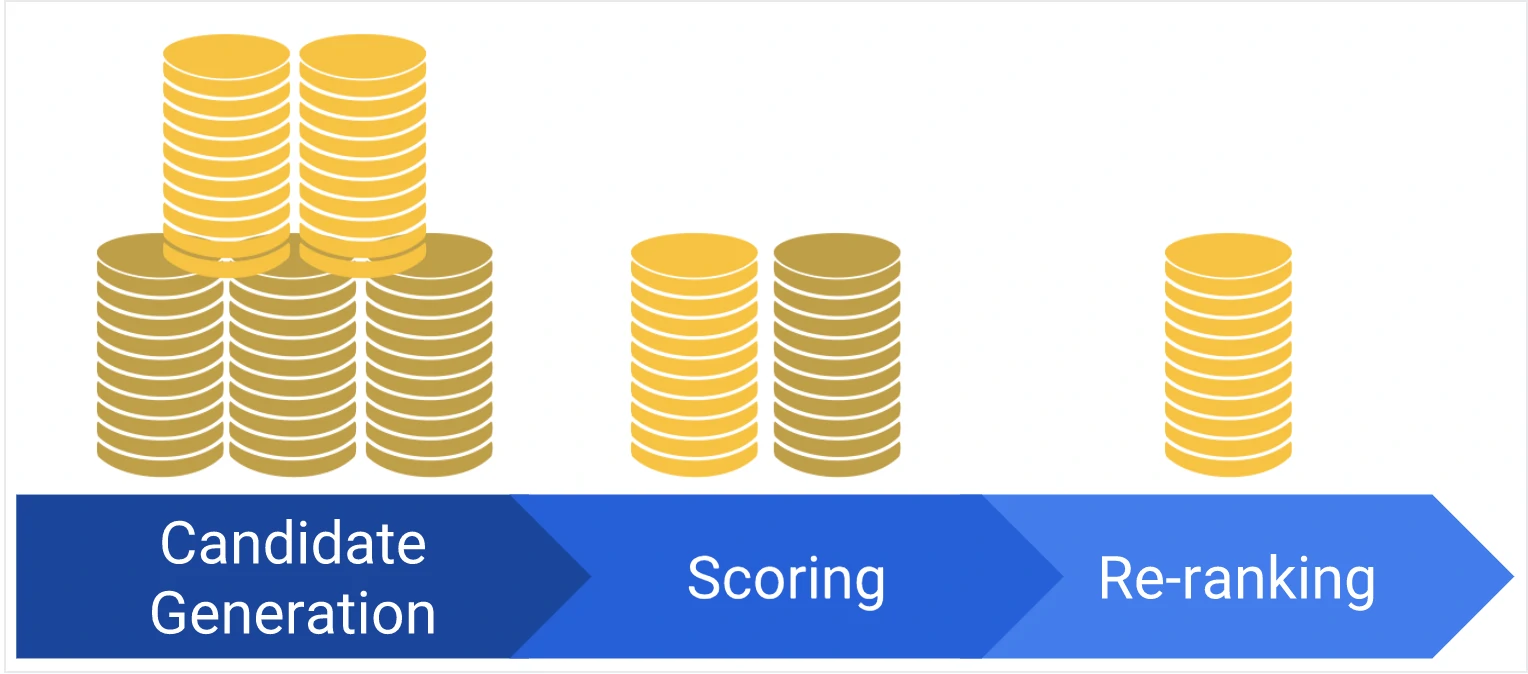
- Candidate Generation: starting with a vast corpus and generating a smaller subset of candidates.
- Scoring: the model ranks the candidates to select a smaller, more refined set of documents.
- Re-ranking: This final step refines the recommendations.
We will discuss deep more about this framework at this page
Market Basket Analysis
- Market basket analysis scrutinizes the products customers tend to buy together, and uses the information to decide which products should be cross-sold.
- Market basket analysis has the objective of identifying products, or groups of products, that tend to occur together (are associated) in buying transactions (baskets).
- A store could use this information to place products frequently sold together into the same area.
- An ecommerce/online shop merchant could use it to determine the layout of their catalog and order form.
- Direct marketers could use the basket analysis results to determine what new products to offer their prior customers.
- It can also be used to improve the efficiency of a promotional campaign
- Market basket analysis mainly works with the ASSOCIATION RULE {IF} -> {THEN}.
- IF means Antecedent: An antecedent is an item found within the data
- THEN means Consequent: A consequent is an item found in combination with the antecedent.
- There are few terminologies that we need to cover: Support, Confidence, and Lift
- Support: It measures the frequency of the association rule in the data.
- The number of transactions with combined items / Total number of transactions.
- A 3% support would mean that 3 out of 100 sales include the two mentioned items.
- Cofidence: Confidence measures how strong an association rule is.
- count of transactions with combined items / count of transactions with single item
- A 40 % confidence would mean that 4 out of 10 sales transaction of x include y
- Lift: is the ratio of confidence to expected confidence.
- (Confidence) / (# Transactions with single item / # Total Transactions)
- Expected confidence is the confidence divided by the frequency of the “consequent” condition. Lift tell us how much better a rule is at predicting the result than just assuming it in the first place.
- Support: It measures the frequency of the association rule in the data.
Association Rule Algorithm
Apriori Algorithm
- It helps to find frequent itemsets in transactions and identifies association rules between them.
- The method employs a “bottom-up” strategy, in which frequent subsets are expanded one item at a time (candidate generation), and groups of candidates are checked against the data.
- The limitation of the Apriori Algorithm is frequent itemset generation. It needs to scan the database many times, leading to increased time and reduced performance as a computationally costly step because of a large dataset. It uses the concepts of Confidence and Support.
FP-Growth / Frequent Pattern Growth Algorithm (FPGA)
- The FP growth algorithm represents data in the form of an FP tree or Frequent Pattern, hence it is a method of mining frequent itemsets.
- A Frequent Pattern Tree is a tree structure that is made with the earlier itemsets of the data.
- The main purpose of the FP tree is to mine the most frequent patterns. Every node of the FP tree represents an item of that itemset. The root node represents the null value, whereas the lower nodes represent the itemsets of the data. While creating the tree, it maintains the association of these nodes with the lower nodes, namely, between item sets.
AIS Algorithm
SETM Algorithm
Classic Recommendation Engine model
Popularity-based / package-based
Provide items based on:
- New arrivals
- Best sellers
- Top reviewed/ top rated
- Sales and offers
- Trending items
Purpose:
- Cold start
- Fallback strategy
Knowledge based
Provide item recommendations based on a user’s needs and relevant information. Recommends utilize for rarely bought items.
| Pros | Cons |
|---|---|
|
|
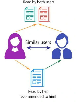
Collaborative Filtering
Recommends items to an individual based on the items purchased or consumed by other users with shared interests. Recommends items to a user based on analysis of similar users and their preferences, past purchases, ratings or other general behavior. History of the user plays an important role.
-
Item based Recommendations are generated by considering the preferences in the user’s neighborhood.
User-based collaborative filtering is done in two steps:
- Identify similar users based on similar user preferences
- Recommend new items to an active user based on the rating given by similar users on the items not rated by the active user.
-
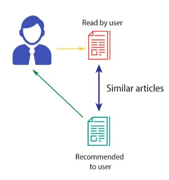
User based The recommendations are generated using the neighbourhood of items. Unlike user-based collaborative filtering, we first find similarities between items and then recommend nonrated items which are similar to the items the active user has rated in past.
Item-based recommender systems are constructed in two steps:
- Calculate the item similarity based on the item preferences
- Find the top similar items to the non-rated items by active user and recommend them
main methods:
- Score matrix
- Similarity score
The main distinction between the two methods lies in the selection of input.
- Item-based filtering first takes a given item, finds users who liked that item, and then retrieves other items that those users liked.
- User-based filtering first takes a selected user, finds users similar to that user based on similar ratings, and then recommends items that the similar users also liked.
In reality, item-based and user-based collaborative filtering tend to produce similar item recommendations, but user-based filtering can be more accurate for datasets that have a large number of users with esoteric interests.
| Pros | Cons |
|---|---|
|
|
- Models
- Truncated SVD
- The Naive Bayes Classifier
- Nearest Neighbors
Content-based Filtering
Recommends items based on user-item profile and metadata. Provide recommendations based on similar item attributes and the profile of an individual user’s preferences.
| Pros | Cons |
|---|---|
|
|
- Mechanism of Content-Based Filtering
- Examining the attributes or features of items, such as textual descriptions, images, or tags.
- Constructing a profile of the user’s preferences based on the attributes of items they have engaged with.
- Recommends items similar to those the user has previously interacted with, drawing on the similarity between the item attributes and the user’s profile.
- Models
- KNN (Basic, means, z-scores)
- The Naive Bayes Classifier
- Main methods
- Items profile
- User profile and preferences
- Document vector (NLP)
- Similarity score
-
Examples
Context-aware based Filtering
similiar with content-based recommendations with additional of filter out for current context.
| Pros | Cons |
|---|---|
|
|
Main methods
- Items profile
- User profile and preferences
- Document vector (NLP)
- Similarity score
How to implement context:
- Post-filtering approaches
- Context information is applied to the user profile and product content.
- Filter out all the non-relevant features, and final personalized recommendations are generated on the remaining feature set.
- Pre-filtering approaches
- Personalized recommendations are generated based on the user profile and the product catalogue, then the context information is applied to filter out the relevant products to the user for the current context.
Hybrid recommenders
This type of recommendation engine is built by combining various recommender systems to build a more robust system.
The most common approaches followed for building a hybrid system are as follows:
- Weighted method
- the final recommendations would be the combination, mostly linear, of recommendation results of all the available recommendation engines.
- Mixed method
- mix results from all the available recommenders.
- Switching method
- Cascade method
- Recommendations are generated using collaborative filtering. The contentbased recommendation technique is applied and then final recommendations / a ranked list will be given as the output.
- Feature combination method
- Combine the features of different recommender systems and final recommendation approach, is applied on the combined feature sets. I.e. combine both User-Item preference features extracted from content based recommender systems and, User-Item ratings information.
- Feature augmentation
- Meta-level
| Pros | Cons |
|---|---|
|
Example:
- content-based model to compute the 25 most similar items
- Compute the predicted ratings that the user might give these 25 items using a collaborative filter
- Return the top 10 items with the highest predicted rating
Other components to build recommendation
- Demographic
- Constraint-limited (Hype or FOMO)
- Time-sensitive
- Location-based
- Group-based
- Social structure / network
Prediction / Scoring model
| Pros | Cons |
|---|---|
|
|
Classic algorithms
- Baseline
- NormalPredictor
- SVD and SVD++ algorithm
- For handle very large user-rating with high data sparsity
- SVD++ is an enhancement of standard matrix factorization techniques designed for collaborative filtering in recommender systems.
- SVD++ also incorporates implicit feedback (e.g., which items a user has interacted with but not rated), leading to improved prediction accuracy.
- SVD++ builds upon the standard MF model by incorporating implicit feedback, represented as items the user has interacted with (e.g., viewed, purchased, clicked).
- Non-negative Matrix Factorization
- Fill the missing data and uses matrix decomposition methods and multiply back to get the approximate original matrix and learn the optimal factor vectors.
- The algorithm performs a decomposition of the (sparse) user-item feedback matrix into the product of two (dense) lower-dimensional matrices. One matrix represents the user embeddings, while the other represents the item embeddings.
- In essence, the model learns to map each user to an embedding vector and similarly maps each item to an embedding vector, such that the distance between these vectors reflects their relevance.
- Mechanism:
- MF first randomly initializes the user and item embedding matrices
- Iteratively optimizes the embeddings to decrease the loss between the Predicted Scores Matrix and the Feedback Matrix using loss function.
- Loss Function
- This loss function will minimize the squared distance over the observed ⟨user,item⟩ pairs, between the predicted and actual feedback values over all pairs of observed (non-zero values) entries in the feedback matrix.
- Keep in mind that there are unobserved pairs, these condition could be translate as unobserved interactions. This lack of interaction doesn’t necessarily mean that the user dislikes the content—it could simply indicate that they haven’t encountered it yet.
- By treating unobserved pairs as negative data points and assigning them a zero value in the feedback matrix, we can minimize the squared Frobenius distance between the actual feedback matrix and the predicted matrix.
- A more balanced approach is to use a weighted combination of squared distances for both observed and unobserved pairs. This method combines the advantages of both approaches. The first summation calculates the loss for observed pairs, while the second summation accounts for unobserved pairs, treating them as soft negatives.
- Next, we could also need to weight the observed pairs carefully. For example, frequent items (such as extremely popular YouTube items) or frequent queries (from heavy users) may dominate the objective function. To correct for this effect, training examples can be weighted to account for item frequency.
- For new users or items, the concept of fold-in is apply.
- Fold-in is the process of incorporating a new user or item into the factorization framework without retraining the entire model. Instead of learning all embeddings from scratch, the existing item embeddings V (which are precomputed during training) are held fixed, and only the embedding for the new user (or item) is optimized.
- For a new user, the algorithm initializes their embedding vector randomly and optimizes it iteratively to minimize the loss between their known interactions (with items) and the predictions made by the model using the fixed item embeddings. Similarly, for a new item, the user embeddings are fixed, and the new item’s embedding is adjusted.
- Stochastic Gradient Descent (SGD)
- SGD is a general-purpose optimization algorithm widely used to minimize loss functions in machine learning and deep learning.
- Steps in SGD:
- Compute Gradient: For each iteration, SGD calculates the gradient of the loss function with respect to the parameters based on a randomly chosen subset of the data.
- Parameter Update: Parameters are updated by moving in the direction opposite to the gradient by a small step size, also known as the learning rate.
- Repeat: This process continues until convergence or for a predefined number of iterations.
- Weighted Alternating Least Squares (WALS)
- the loss function is quadratic in each of the two embedding user and item matrices, i.e., U and V. WALS performs MF in an alternating fashion: it iteratively fixes one of the two embedding matrices (such as user or item embeddings) and solves a least squares optimization problem for the other. This alternating approach is repeated until convergence, enabling WALS to handle weighted MF objectives.
- This is an efficient algorithm that is particularly well-suited for MF, since it effectively deals with large, sparse matrices common in recommendation systems. WALS can be distributed across multiple nodes, making it efficient for large-scale data.
- Optimization Process in WALS:
- Fix One Matrix: Start by fixing one matrix, say the user matrix, and then optimize the other matrix (e.g., the item matrix). Put simply, WALS works by alternating between fixing one matrix and optimizing the other:
- Fix U and solve (i.e., optimize) for V.
- Fix V and solve (i.e., optimize) for U.
- Alternate: After solving for the item matrix, fix it and solve for the user matrix.
- Iterate Until Convergence: Continue alternating between the two matrices until the objective function converges. Each step can be solved exactly by solving a linear system, leading to efficient convergence.
- Fix One Matrix: Start by fixing one matrix, say the user matrix, and then optimize the other matrix (e.g., the item matrix). Put simply, WALS works by alternating between fixing one matrix and optimizing the other:
- SlopeOne algorithm
- WARP (Weighted Approximate-Rank Pairwise)
- BPR (Bayesian Personalized Ranking)
Machine Learning
- Classification models
- Logistic regression
- Logistic matrix factorization
- SVM
- Tree based model
- Ensemble model
- LightGBM / XGBoost
- Clustering techniques
- KNN (Basic, means, z-scores)
- It assigns a class to a particular data point by a majority vote of its k nearest neighbors. The data point is assigned the class that is the most common among its k-nearest neighbors. In the case of regression, it computes the average value for the target variable based on its k-nearest neighbors.
- K-NN is non-parametric and lazy in nature. The former means that k-NN does not make any underlying assumptions about the distribution of the data. In other words, the model structure is determined by the data.
- K-means clustering
- Co-clustering
- KNN (Basic, means, z-scores)
Deep Learning
- Neural Collaborative Filtering
- Wide & Deep
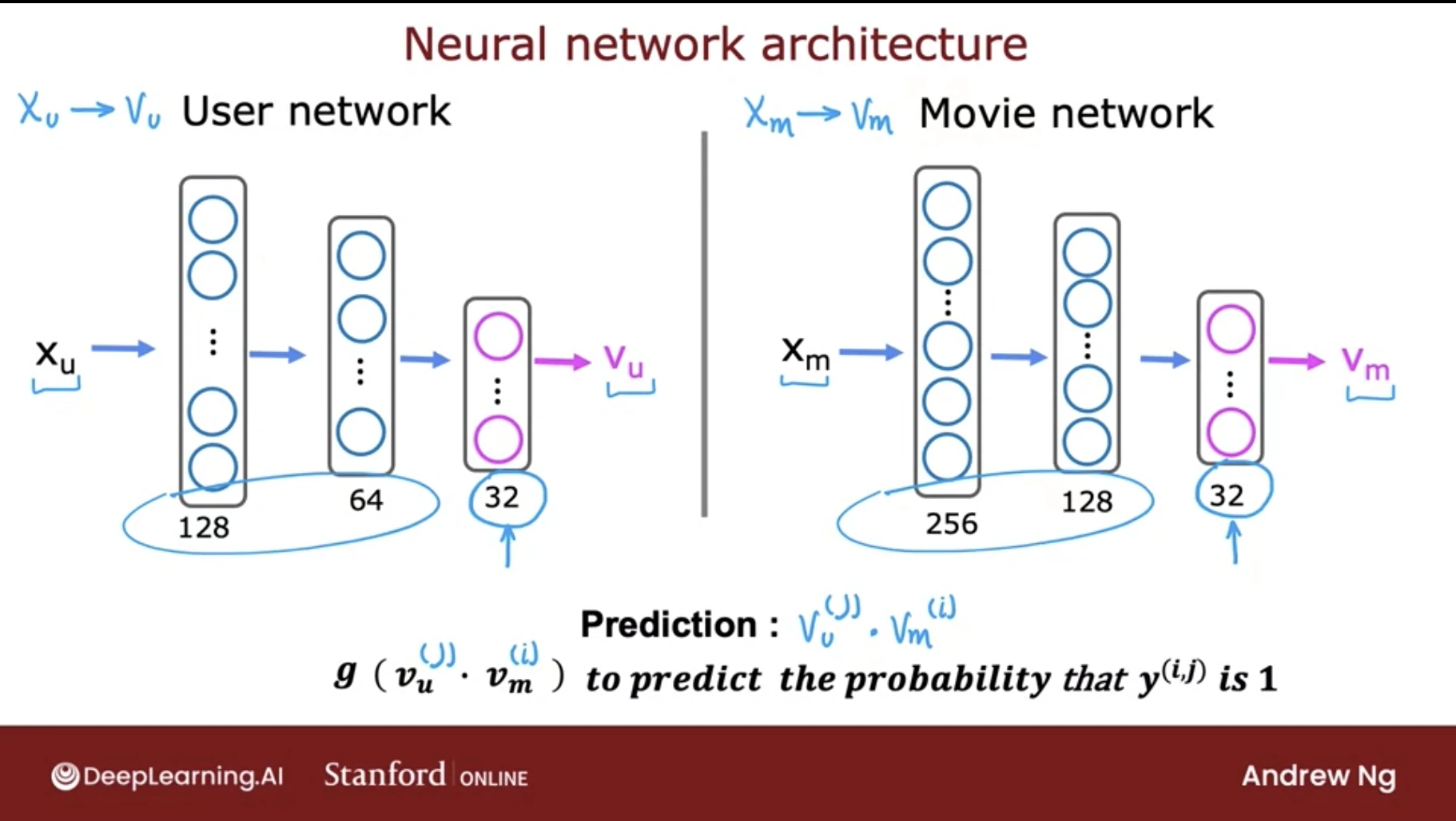
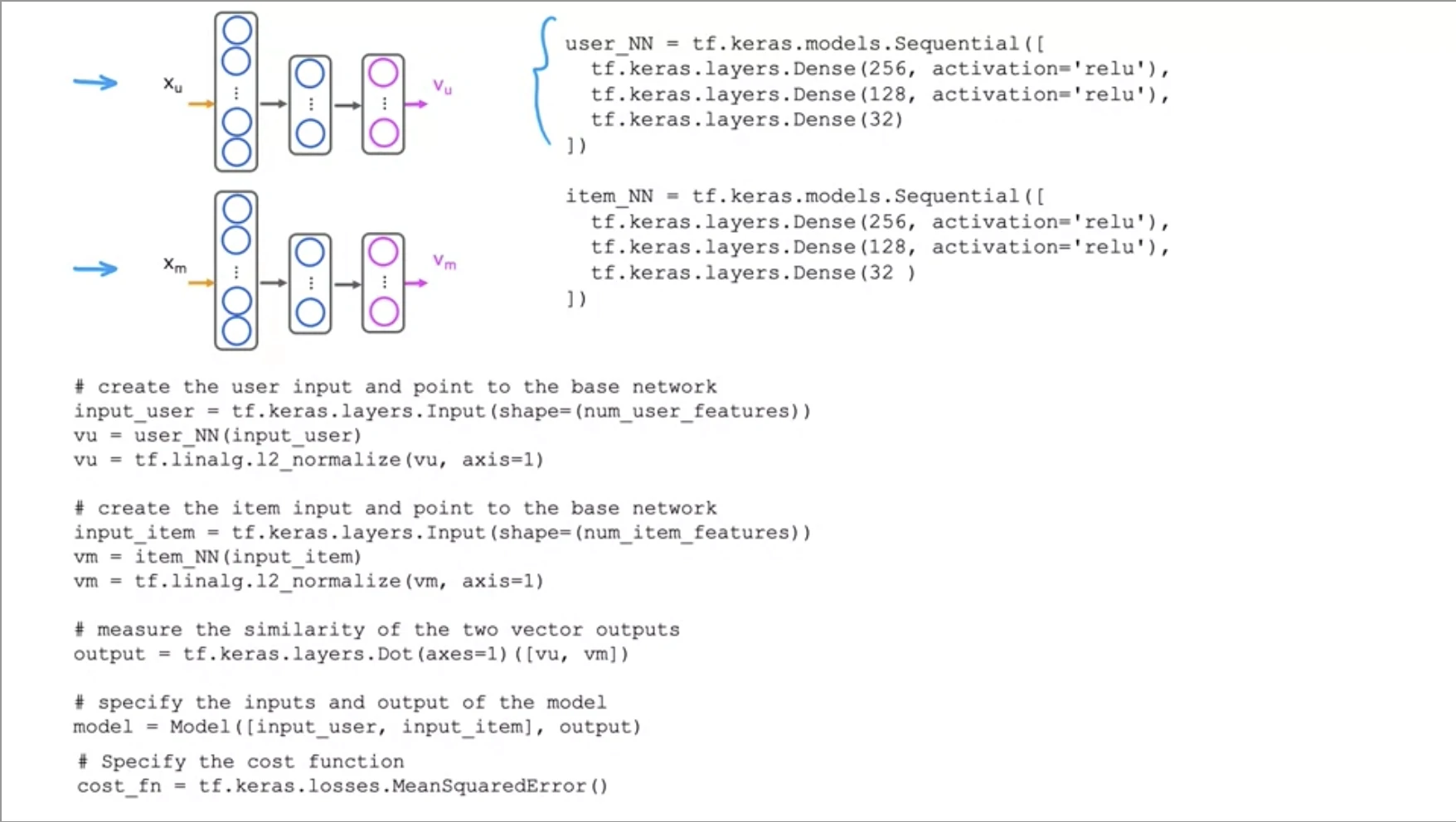
- Two-Tower Models (User tower + Item tower)
-
are primarily used for retrieval stage, the goal of retrieval is to efficiently select a small subset of potentially relevant items from a huge catalog (often millions).
- Mechanism
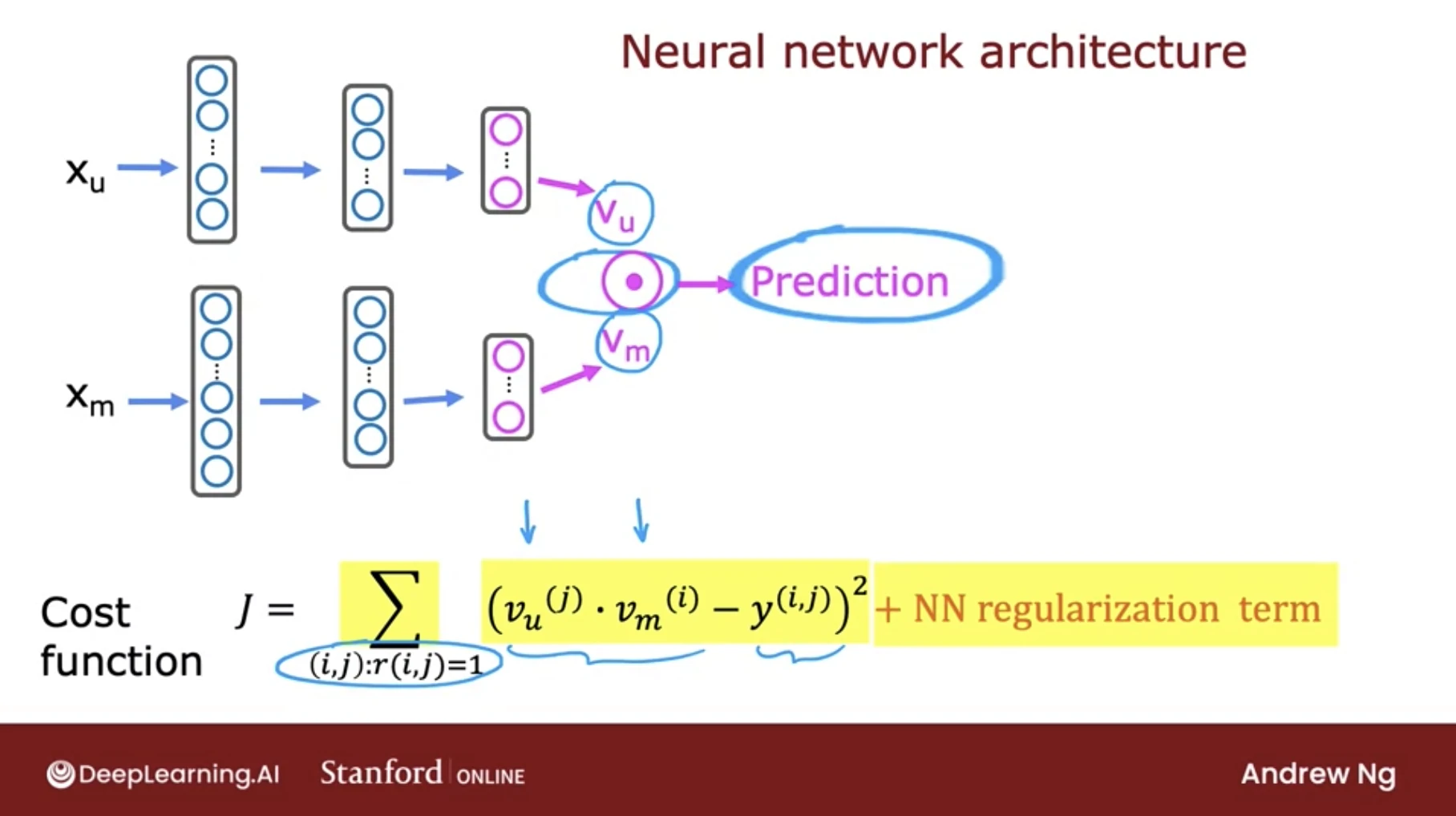
- The two-tower model consists of two neural networks (towers): one encodes the user (using features like demographics, interaction history, etc.), and the other encodes the item (using features like content, metadata, etc.).
- Both embeddings are projected into the same latent vector space, and relevance is computed via a simple similarity measure, usually the dot product or cosine similarity:
score(u,i) = eu ⋅ ei
- Because this similarity can be computed efficiently, approximate nearest neighbor (ANN) search can quickly retrieve the top candidate items.
- The trained embeddings of query and item towers are stored for fast retrieval.
- Implementation
- Collaborative filtering
- In collaborative filtering, recommendations are learned from user–item interaction data (e.g., clicks, views, purchases) without needing explicit content features.
- The user tower and item tower each learn embeddings that reflect behavioral patterns:
- User tower: learns from user IDs and possibly historical interactions.
- Item tower: learns from item IDs and co-occurrence patterns.
- These embeddings capture collaborative signals—items liked by similar users end up close in embedding space.
- Content-based filtering (possible use):
- Two-tower models can also incorporate content features directly:
- User tower: could use profile data, demographics, or textual preferences.
- Item tower: could use metadata, descriptions, or image/text embeddings.
- This makes the model suitable when interaction data is sparse (cold start problem).
- Two-tower models can also incorporate content features directly:
- Collaborative filtering
-
- Transformer-based session models
Graph-Recommendation Engine model
- Graph-based recommender
Learning-to-Rank Models
- LambdaMART
- RankNet
- XGBoost ranking
- LightGBM ranking
Data Understanding
What kind of data will we use?
Each objective dependent on user information data. At a minimum, this includes transaction history, behavioral and activity data, and demographic or profile attributes.
For a personalized recommendation system, this dependency increases. We must have structured item metadata and real-time context—capturing the relationship between the user, the item, and the current situation in which a decision is made.
These data could come from internal and external sources. That should be considered some trade-off between them and cost-benefit.
- Internal data
- Transactional data
- Logging and tracker data
- User profile data
- External data
- 3rd party data
- Governance data
- Public data
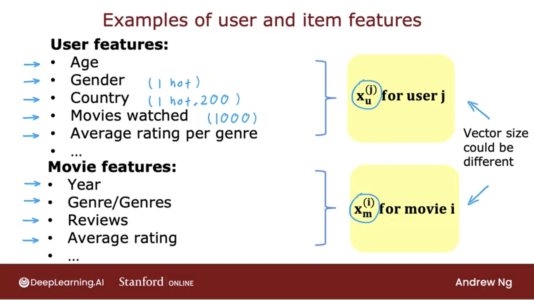
Item and Context Information
- Metadata item (Enables semantic matching)
- Description (image / text embeddings)
- Quality
- Brand
- Product category
- Category hierarchy
- Popularity (A social proof and baseline relevance data)
- Total sold and Latest sold item
- Product category affinity
- Target market
- Promotion
- Accessibility (Users profile and their segment)
- Location
- Channel
- Delivery constraints
- Monetary
- Price and Price sensitivity
- Margin
- Revenue objectives
- Inventory (supports operational alignment)
- Stock availability
- Delivery constraints
- Context (to get specific conditions)
- Time (Captures temporal patterns)
- Time-of-day / week / month effects
- Payday
- Holiday
- Season (for cyclical demand)
- Campaign / promotion
- Popular items or events
User Information
- Transactional (actual economic behavior)
- Past purchases
- Average order value (AOV)
- Monetary (with or w/o limit days)
- Recency
- Frequency
- Age-recency
- Discounts used
- Payment method
- Activity / behavior (Captures real engagement or implicit data)
- Page, Category or Product views, searches
- Login frequency
- Session duration
- Click-throughs
- Time since last activity
- Time on product page
- Checkout started
- Device type
- Add-to-cart
- Dwell time
- Scroll depth
- Demographic / profile (Users profile and their segment)
- Age and Account age
- Sex / Gender
- Location
- Target market / user categories
- Purchasing power
- Preference input (Explicit data from users)
- Keywords search
- Preference input
- Reviews
- Likes or ratings
- Wishlist / save actions
- Add-to-cart events
- Marketing & Exposure (Controls for influence bias)
- Mail Opened / clicked
- Ad impressions
- Coupon received / redeemed
Data Preparation
Do feature engineering to give more efficient features
To give more useful information, help the models learn real behavior, and avoid amplify noise, data Preparation is crucial and mandatory foundations for both objectives. In example:
Common feature engineering
- Weight score
- RFM
- Categorization
- Standardization
- Grouping / Clustering
- Feature selection
- Feature importance
- PPScore
- Temporal Aggregations
- Rolling windows (7, 14, 30, 90 days)
- Decay-weighted counts
- Day of week
- Dimensionality reduction
- PCA, t-SNE
- Label data selection
- Multi-class vs binary-class
- Text processing
- Text vectorization
- Similarity techniques
- Euclidean distance
- Cosine, Jaccard similarity
- Pearson correlation coefficient
Specific feature engineering
- Item Popularity
- Global popularity
- Trending score
- Recent sales velocity
- Conversion Ratios
- Add-to-cart ÷ views
- Purchases ÷ sessions
- Discounted purchases ÷ total purchases
- User Embeddings
- Session embeddings
- Product embeddings
- User–item interaction vectors
- Behavioral Intensity
- Product views (7 / 14 / 30 days)
- Add-to-cart count
- Checkout initiation count
- Implicit Feedback Signals
- View = weak signal
- Cart = strong signal
- Purchase = strongest signal
- Last interaction timestamp
- Count of interactions in last N days
- Decay-weighted interaction score
- User Affinity
- Top categories viewed
- Average viewed price vs purchase price
- Brand affinity score
- Category affinity vector
- Brand preference score
- Price sensitivity
- Temporal Features
- Days since last cart action
- Time since last promo exposure
- Day-of-week / hour-of-day
Labeling
- explicit Feedback Labels
- Ratings
- Reviews
- Implicit Feedback Labels
-
Binary or weighted signals: Label is interaction strength, not explicit rating.
Action Label Weight View 1 Add-to-cart 3 Purchase 5
-
- Pairwise Ranking Labels
- For ranking models used in BPR and Learning-to-rank with this formula
(user, purchased item) > (user, viewed but not purchased item)
- For ranking models used in BPR and Learning-to-rank with this formula
Evaluation
Before Deployment
- Benchmark
- Cost and Benefit (comparing TP, FP, TN, FN in the confusion matrix)
- How much lost that generate if we get false positives and negatives?
- How much revenue would that generate if we got a true positive?
- Business-Level Evaluation
- Revenue uplift @ K; how to allocate a constrained budget with the highest return.
- ROI vs random targeting
- Metrics evaluation
- Precision@K; it focus on False Positives, to see how many actually buy?
- Recall@K; it measures coverage of user intent.
- NDCG@K (Normalized Discounted Cumulative Gain); it focus on Correct items with correct order.
- MAP@K; “Across users, how early do we surface relevant items?”
- Numeric evaluation
- RMSE
- MAE
- Classification evaluation
- Precision-Recall
- Precision
- Recall
After Deployment
- Online evaluation methods
- A/B testing
- Two prediction models randomly alternate between users so comparisons can be formed from the results of Group A and Group B. Users in Group A might be fed collaborative-based filtering recommendations, while users in Group B might be exposed to contentbased recommendations.
- Typically require a thousand or more users to accurately assess the performance of one recommender system model over another.
- The performance of the systems can be evaluated based on numerous metrics.
- A/B tests should only test one variable at a time.
- The advantages:
- A/B testing over user studies are scalability and relevance.
- A/B test results are highly relevant as they capture genuine interactions between the end-user and the recommended item(s)
- Users are generally impervious to the fact that a website is conducting live A/B testing and aren’t coerced to select a recommended item as they might in a user study.
- A/B testing
- User Engagement/Business Metrics
- click-through-rates (CTR)
- Conversion rate
- Revenue per session
- Add-to-cart rate
- ROI measurement
- HR (hit ratio)
- Session Length
- Dwell Time
- Bounce Rate
- Hit Rate
- Recognizes items in the top-N list that the user has rated in the past and is divided by the number of items in the list.
- Generate top-N recommendations for all of the users. If one of the recommendations in a users’ top-N recommendations is something they actually rated, we consider that a “hit”. We actually managed to show the user something that they found interesting enough to watch on their own already, so we’ll consider that a success. Just add up all of the “hits” in our top-N recommendations for every user, divide by the number of users, and that’s our hit rate.
- It’s a much more user-focused metric
- Average reciprocal hit rate (ARHR)
- This metric is just like hit rate, but it accounts for where in the top-N list our hits appear (A weighting system that takes into account the item’s placing in the top-N list). So, we end up getting more credit for successfully recommending an item in the top slot than in the bottom slot.
- This is a more user-focused metric, since users tend to focus on the beginning of lists and it depends a lot on how our top-N recommendations are displayed.
- The only difference is that instead of summing up the number of hits, we sum up the reciprocal rank of each hit. So, if we successfully predict a recommendation in slot 3, that only counts as 1/3. But a hit in slot 1 of our top-N recommendations receives the full weight of 1.0.
- Cumulative hit rank
- it throws away hits if our predicted rating is below some threshold. Which means that we shouldn’t get credit for recommending items to a user that we think they won’t actually enjoy.
- Thus, we shouldn’t count the value below threshold.
- Rating hit rate (rHR)
- Hit rate that breaks it down by predicted rating score.
- It can be a good way to get an idea of the distribution of how good our algorithm thinks recommended movies are that actually get a hit.
- Ideally we want to recommend movies that they actually liked, and breaking down the distribution gives us some sense of how well we’re doing in more detail.
- Coverage
- That’s just the percentage of possible recommendations that our system is able to provide.
-
% of <user,item> pairs that can be predicted.
- This measurement is a trade-off with accuracy, If we enforce a higher quality threshold on the recommendations we make, then we might improve our accuracy at the expense of coverage (serendipity).
- Coverage can also be an important to watch, because it gives us a sense of how quickly new items in our catalog will start to appear in recommendations.
- Diversity
- A measure of how broad a variety of items in our recommender system.
-
Diversity = 1 - S ; S = avg similiarity between recommendation pairs
- This metrics is trick due to it behavior to give very high deiversity by just recommeding completely random items. Thus, it need to co-exist with other metrics.
- Novelty
- Is a measure of how popular the items are that we are recommending.
-
mean popularity rank of recommended items
- Again, just recommending random stuff would yield very high novelty scores, since the vast majority of items are not top-sellers.
- Churn
- How often do the recommendations for a user change?
- Churn can measure how sensitive our recommender system is to new or existing user behavior.
- Again, just recommending random stuff would yield very high churn scores.
- Responsiveness
- How quickly does new user behavior influence our recommendations? If we rate a new movie, does it affect our recommendations immediately.
- More responsiveness would always seem to be a good thing, but in the world of business we have to decide how responsive our recommender really needs to be – since recommender systems that have instantaneous responsiveness are complex, difficult to maintain, and expensive to build.
- We need to strike our own balance between responsiveness and simplicity.
- User Studies / Perceived quality
- Another thing we can do is just straight up ask our users if they think specific recommendations are good.
- In practice though, it’s a tough thing to do. Users will probably be confused over whether we asking them to rate the item or rate the recommendation, so we won’t really know how to interpret this data.
- It also requires extra work from our customers with no clear payoff for them, so we’re unlikely to get enough ratings on our recommendations to be useful.
- Evaluating Candidate Ranking
- MRR (Mean Reciprocal Rank)
- MAP (Mean Average Precision)
- NDCG (Normalized Discounted Cumulative Gain)
###
How to choose recommendation model
General phase
- Phase 1: General recommendation engines
- Popularity-based / package-based
- Knowledge based (for rarely bought items)
- Collaborative Filtering
- Phase 2: Personalized recommendation engines
- Content-based
- Context-based
- Hybrid recommenders
- Deep and Machine learning model
- Learn to Rank Model
- Phase 3: Futuristic recommendation engine
- more personal data
- agentic ai
Specific phase
(First phase) For a single product category such as skincare, we should start with a classical recommendation approach. In example focus on content-based and context-aware recommenders to deliver relevant, personalized product suggestions grounded in user needs and usage conditions.
(Second phase) we can extend value through complementary product recommendations (to create cross-sell and upsell) by applying market basket analysis to identify items that are naturally purchased together.
(Third phase) With sufficient data maturity and feedback loops in place, we then progress to predictive models that enable more advanced decisioning, such Learning-to-Rank Models.
Privacy and Ethics
- How to collect, manage, process, usage data privacy and sensitive information.
- How comply with local and global regulation.
- How to manage bias result from the model.
- Consideration of consent, alertness to bias, and protecting data from becoming deanonymized.
- To minimize legal risk and other public repercussions is to scrutinize what information is fed to the recommendation engine in the first place.
- Encourage transparency internally and ensure that relevant departments such as upper management and legal teams are aware of the variables chosen to generate recommendations as well as the composition of what is recommended to users as output.
Deployment
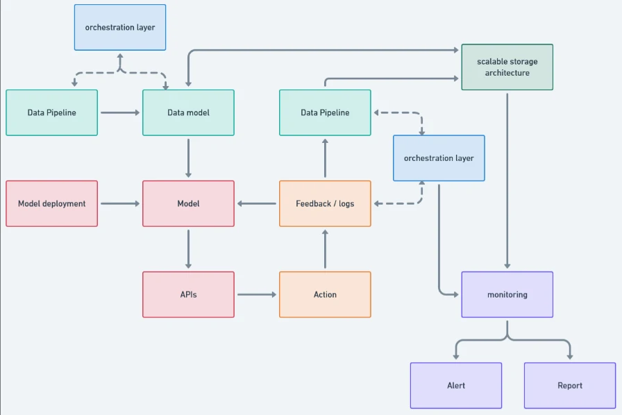
- Design a formal data model that defines relationships, enforces standards, and creates a shared language across the system.
- The data model must be backed by a scalable storage architecture aligned with serving needs. Different workloads require different stores. (i.e. postgres - offline analytics and feature generation, redis - online inference and real-time access).
- On top of this, we need an orchestration layer to automate configuration, execution, and coordination across the system. The choice of orchestrator depends on architectural decisions, such as workflow orchestration for batch processes (e.g., Airflow) and event-driven systems for real-time data flows (e.g., Kafka).
- Model deployment should follow the same architectural discipline. Models should be containerized and deployed via cloud or hybrid infrastructure to enable repeatable CI/CD processes, versioning, and controlled rollbacks.
- To operationalize model outputs, we expose them through well-defined APIs and integrate them directly into digital touchpoints such as websites and mobile applications.
- Using Feedback Loop system, we could systematically capture user interactions, model inference outputs, and online evaluation data, then align them back into the data model, storage layer, and orchestration workflows.
- We establish monitoring and governance as first-class components. This includes technical monitoring (feature drift, model performance, latency, SLA compliance) and business monitoring (ROI, conversion uplift, and downstream impact). The objective is fast detection and decisive response, not retrospective reporting.
- All of these components should be integrated into a unified CI/CD pipeline. This is what enables scalable deployment, controlled experimentation, and sustainable maintenance as the system evolves.
Strategic Tips
- A key goal of recommender systems is item discovery
- Recommendation effectiveness is highly dependent on the use case and the presentation context. The same model can perform well or fail entirely depending on where, when, and how recommendations are surfaced in the user journey.
- A core objective of recommender systems is item discovery, not immediate conversion. Users often require multiple exposures before developing intent or completing a target action.
- Recommendations should be evaluated over repeated exposure. A minimum exposure policy—typically three or more impressions—should be applied before concluding that an item is a poor match.
- Not all eligible items should be shown. Only the top-N recommendations should be surfaced, filtered by contextual constraints such as user location, channel, inventory availability, and UI placement.
- For specialized product categories (such as skincare), recommendation logic must differ fundamentally from broad, multi-category e-commerce systems. E.I. The strategy should explicitly separate recommendation paths for new versus existing customers.
- New customers (cold start): When profile and behavioral data is unavailable, recommendations must rely on item metadata and explicit preference capture. This can include user-declared inputs (e.g., skin condition, lifestyle, usage goals) and, where appropriate, computer vision or diagnostic tools to infer user needs. These data enable content-based, context-aware, or hybrid recommendations.
- Existing customers (known users): For users with prior product usage, recommendations should avoid repeating the same product category. If the user is already satisfied with a product, the system should prioritize cross-sell or upsell strategies using complementary items to extend value and deepen product adoption.
- There’s a concept of user trust in a recommender system – people want to see at least a few familiar items in their recommendations that make them say, “yeah, that’s a good recommendation for me. This system seems good.” If we only recommend things people have never heard of, they may conclude that our system doesn’t really know them, and they may engage less with our recommendations as a result.
- Consider the condition that the recommended items were too similar to items the user had already purchased or consumed in the past. Rather than being recommended a near-identical item, the user perhaps prefers some variety in their recommendations.
- Popular items are usually popular for a reason – they’re enjoyable by a large segment of the population, so we would expect them to be good recommendations for a large segment of the population who hasn’t read or watched them yet. If we’re not recommending some popular items, we should probably question whether our recommender system is really working as it should.
- We need to strike a balance between familiar, popular items, and what we call “serendipitous discovery” of new items the user has never heard of before. The familiar items establish trust with the user, and the new ones allow the user to discover entirely new things that they might love.
- NONE of the metrics we’ve discussed matter more than how real customers react to the recommendations our produce, in the real world. We can have the most accurate rating predictions in the world, but if customers can’t find new items to buy or watch from our system, it will be worthless from a practical standpoint.
-
There is a real effect where often accuracy metrics tell us an algorithm is great, only to have it do horribly in an online test. YouTube studied this, and calls it the “surrogate problem.” Accurately predicted ratings don’t necessarily make for good video recommendations.
There is more art than science in selecting the surrogate problem for recommendations.
It means that we can’t always use accuracy as a surrogate for good recommendations.