Scoring for Customers
scoring
- Scoring for Customers
- Goals
- Unit of Analysis and Data Scope
- Define the matrix
- Customer’s journey from province to trx in rules
- Derivative matrics
- Sample Cases
- How we calculate the score?
- Bayesian Approximation
- Custom Scoring
- Combining score status & score revenue
- Proposed Customer Segments
- So, What next? - Probable Action items
- Illustrative Action Direction
- Feature Expansion
- Integration with RFM Framework
- Operational Application
Goals
How to score customers to determine their performance.
We’ve approved ~12000 customers across 146 locations in 22 provinces. Of those, 7000 have actually transacted. However, we can only measure the first payment default (FPD) for only 5,000 customers. This creates an immediate measurement gap—risk insights are being derived from a partial and potentially biased subset.
Transaction behavior is uneven. A subset of customers is highly active (20+, 50+, up to 384 transactions), while others are inactive, either recently onboarded (e.g., 2022 cohorts) or one-time users with no follow-up activity. Treat these as distinct behavioral segments, not a single population.
Each transaction falls into one of five states: current (paid before due date), BDR, NPL, write-off (WO), or not yet due. These states form the basis for a scoring matrix that evaluates customer quality through observed loan performance—shifting the focus from raw activity to risk-adjusted behavior.
Unit of Analysis and Data Scope
The analysis focuses on customers with a prior loan application who are currently in an overdue status. Customers with recent loan applications who have not yet reached overdue are excluded to avoid premature or incomplete risk signals.
The primary dataset is sourced from the feedfund_customers table. Detailed payment behavior data has been available since July 2022, which defines the effective observation window for behavioral analysis.
All relevant data sources have been consolidated into a single analytical table for this study, with additional transformations applied where necessary to support downstream modeling and evaluation.
Define the matrix
This deck introduces a set of scoring matrices to evaluate customers’ loan performance. The primary framework, referred to as the transaction status matrix, structures each loan based on its repayment outcome.
| Params | Details |
|---|---|
| DPD (Days Past Due) | Information about how long the transaction has passed the bill payment due date. |
| BDR30 | Transactions with a DPD value greater than 0 up to 30 days. |
| BDR30plus | Transactions with a DPD value greater than 30 up to 90 days. |
| NPL | Transactions with a DPD value greater than 90 up to 180 days. |
| WO | Transactions with a DPD value greater than 180 days. |
The matrix incorporates both active (outstanding) exposures and transactions that have been fully settled within the observation window, ensuring the assessment reflects the full lifecycle of each loan.
A key design choice is the split within the BDR category into BDR30 and BDR30+. This separation is intentional: it distinguishes early-stage delinquency from more severe, persistent delays. To understand the rationale, we need to examine how customers’ transactions distribute across these categories.
Customer’s journey from province to trx in rules
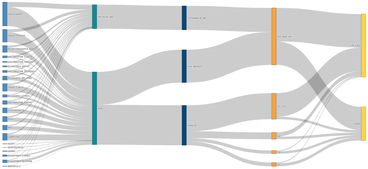
Each line represents a customer’s transaction trail starting from the originating province through to its classification against the defined rules. At a system level, the transaction flow is consistent, with no structural anomalies detected.
What stands out is the composition of outcomes: defaulted transactions (13.5k) exceed non-defaults (11k), indicating that delinquency is not an edge case but a dominant pattern in the portfolio.
Within defaults, the distribution is heavily concentrated in early-stage delinquency. BDR ≤30 days (BDR30) accounts for 8.81k cases, or ~65% of total defaults. More importantly, this segment is largely fulfill the due with 7.98k of these transactions have already been repaid, representing ~60% of total defaults and ~91% of the BDR30 bucket.
If BDR is treated as a single undifferentiated category, it expands to 11.11k transactions; ~82% of all defaults and ~45% of all past-due exposures. This aggregation masks a critical distinction: most “defaults” are short-lived and operational in nature, not structural credit failures.
The decision to split BDR into BDR30 and BDR30+ is therefore behavior-driven. Customers predominantly experience delays within a 30-day window, often linked to timing frictions due to harvest cycles, delayed payments at point of sale, or repayment triggered by maturity reminders rather than an inability to repay.
Derivative matrics
Beyond the transaction status matrix, performance can also be evaluated through a revenue-based lens. Here, we use a revenue matrix anchored on the gross margin generated per transaction.
This approach links credit behavior directly to financial impact. When a transaction defaults, its gross margin is adjusted downward by an associated cost, calibrated to the level of delinquency (DPD). In effect, higher DPD translates into a larger erosion of margin, allowing the model to capture not just whether a default occurs, but how materially it affects profitability.
| Params | Details |
|---|---|
| cost_bdr30 | Cost incurred when a customer makes a payment on BDR30. This amount is 5% of the gross margin of the payment. |
| cost_bdr30plus | Cost incurred when a customer makes a payment on BDR30plus. This amount is 10% of the gross margin of the payment. |
| cost_npl | Cost incurred when a customer makes a payment on an NPL. This amount is 15% of the gross margin of the payment. |
| cost_wo | Cost incurred when a customer makes a payment on a WO. This amount is 20% of the gross margin of the payment. |
| cost_ongoing_due | Cost incurred when a customer has not paid off a transaction within the timeframe mentioned above. The amount is a percentage of the status above, multiplied by the gross margin of the outstanding payment. |
Sample Cases
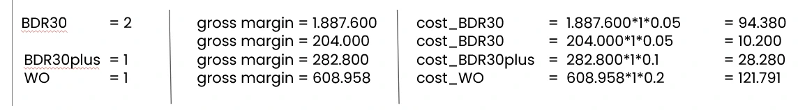
Case no.1 Customer A has made four transactions using our products. All four transactions were in default. This customer paid in full on DPDs 18, 18, 41, and 235. Therefore:
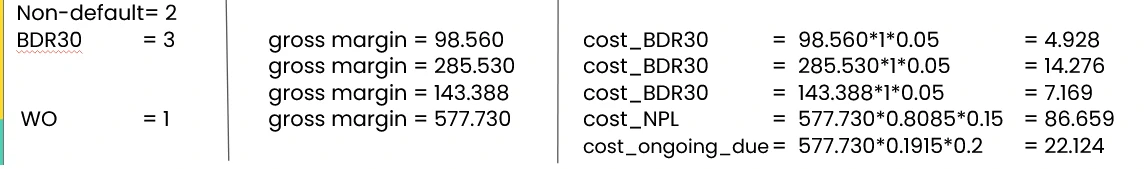
Case no.2 Customer B has made six transactions using our products, with two non-default transactions and four defaults. He paid in full on DPDs 6, 19, 11, and 223. The last transaction was only 80.85% repaid at the time of the NPL. Therefore:
How we calculate the score?
From previous matrices, we created nine main matrices to measure the scores of customers. We categorized them into two categories: status score matrices and revenue score matrices.
| Params | Details |
|---|---|
| total_non_default | Total normal transactions |
| total_at_bdr_30 | Total transactions at BDR30 |
| total_at_bdr_30_plus | Total transactions at BDR30plus |
| total_at_npl | Total transactions at NPL |
| total_at_wo | Total transactions at WO |
| gross_per_GMV | Gross margin ratio per total order amount |
| total_gross_paid | Gross margin of paid transactions, minus cost payments (total gross margin - SUM(cost BDR30+cost BDR30plus+cost NPL+cost WO)) |
| promo | Total promotions used by customers |
| cost_ongoing_due | Total ongoing cost due per gross margin |
We derive two complementary scoring frameworks from these matrices to evaluate customers’ performance. Each matrix operates on a different numerical structure and serves a distinct analytical purpose, so the scoring approach is tailored accordingly.
Status Score Matrix
Matrix characteristics:
- Discrete, ordinal structure (e.g., 1, 2, 3, 4).
- Uneven weight distribution across components—metrics such as total_non_default and total_at_bdr_30 carry higher magnitude relative to total_at_npl and other delinquency states.
Given this structure, a Bayesian approximation approach is appropriate. It stabilizes estimates across varying sample sizes and prevents over-weighting sparse but extreme observations, producing a more reliable representation of customer risk.
Revenue Score Matrix
Matrix characteristics:
- Continuous values with a wide range (denominated in rupiah), requiring normalization—typically via ratios against a baseline such as gross margin.
- Mixed directional impact: components like promo and cost_ongoing_due introduce negative contributions, in contrast to revenue-generating elements.
Given these properties, a custom scoring approach is more suitable. This allows explicit control over normalization, weighting, and the treatment of negative contributors, ensuring the score reflects true economic performance rather than raw monetary scale.
Bayesian Approximation
Bayesian Approximation is a scoring approach grounded in Bayesian inference, where each score reflects both prior assumptions and observed data. It starts with a prior belief, an initial expectation about the object being evaluated, and systematically updates that belief as new evidence becomes available.
In practice, this is implemented using probability distributions (commonly the beta distribution) to model the likelihood of “positive” versus “negative” outcomes. The result is a score that is not purely reactive to observed data, but regularized by prior assumptions, making it more stable especially when observations are limited or uneven.
Scoring Framework (K-scale)
This method operates on a discrete K-scale (e.g., K = 3, 4, 5), where outcomes are grouped into favorable and unfavorable signals.
For example, with K = 5:
- High scores (4–5) → treated as positive signals (upvotes)
- Low scores (1–3) → treated as negative signals (downvotes)
This structure allows us to translate categorical outcomes into probabilistic weights that can be aggregated into a single, robust score.
Application to Status Score Matrix
Mapping the transaction states into the K-scale:
total_non_default → scale 5 → upvote total_at_bdr_30 → scale 4 → upvote total_at_bdr_30_plus → scale 3 → downvote total_at_npl → scale 2 → downvote total_at_wo → scale 1 → downvote
This mapping reflects a clear risk hierarchy: early or resolved delays are still treated as relatively positive signals, while prolonged delinquency and write-offs exert a stronger negative influence. The Bayesian framework then aggregates these signals into a posterior score that balances observed behavior with prior expectations, reducing volatility and improving comparability across customers.
Data Distribution
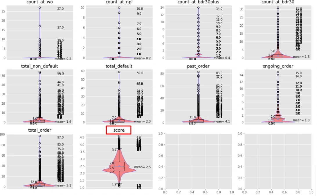
Before applying Bayesian approximation, we examined the underlying data distribution to understand its baseline behavior.
Across parameters, the distributions are broadly similar in shape but exhibit significant outliers. Most observations cluster below 10, yet the upper bounds vary widely, indicating inconsistent exposure and potential skewness across metrics.
After applying the Bayesian scoring (see the “score” distribution), the profile becomes substantially more stable. The values are well-calibrated within the 0–5 scale and show a more uniform spread, with the highest concentration falling in the 2.0–2.5 range. This shift reflects the intended effect of Bayesian smoothing and reducing the influence of extreme values while preserving relative differences in performance.
Sample cases for Bayesian Approximation
We use a set of representative sample cases to validate how the Bayesian scoring behaves in practice. The criteria are broadly aligned with the observed patterns in customers, allowing the framework to be applied without additional calibration.
Four scenario types are tested to different data conditions:
- Single-value parameters (red)
- Uniform distributions (orange)
- Maximum-value concentrations (green)
- Polarized distributions (blue)
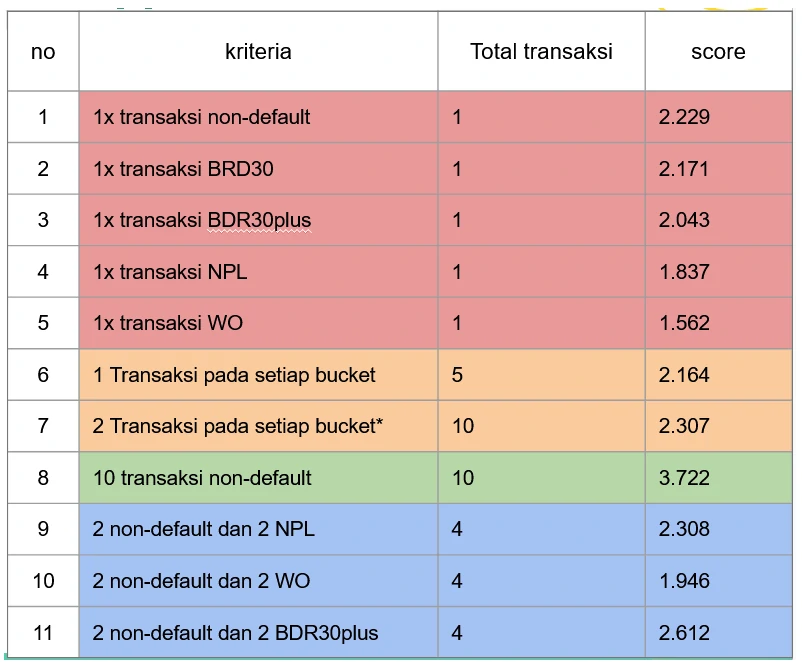
These cases are designed to isolate how each matrix configuration influences the final score. For instance, row 9 produces a score that is nearly identical to row 7. While the total number of transactions differs, row 9 is based on only four transactions, meaning the estimate is still highly influenced by prior assumptions. As a result, it retains upward potential relative to row 7, where the larger volume leads to a more “locked-in” score driven by observed data.
Bayesian Approximation Result
From the distribution, the maximum observed score is 2.23.
This value effectively represents the prior baseline, the score assigned to a customer with minimal history, such as a single non-default transaction. It reflects the model’s starting point before sufficient behavioral data is accumulated.
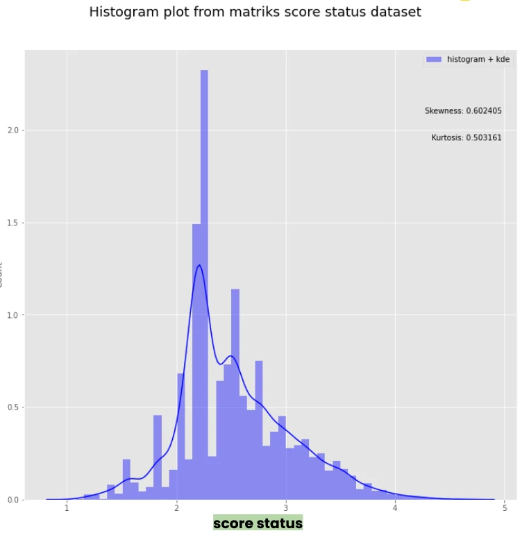
Looking at the broader distribution (right-hand side), scores show a moderate positive skew, with a general tendency toward higher values on the scale. At the same time, a subset of customers falls below the 2.23 threshold, indicating weaker performance driven by a higher proportion of defaulted transactions.
The distribution also exhibits distinct local peaks—notably around scores of 1.5, 2.0, 2.5, and 2.7. These clusters suggest natural groupings in repayment behavior, where customers with similar transaction patterns converge to similar score bands.
When we map the data into an XY scatterplot—transaction volume on the x-axis and status score on the y-axis—the structure becomes more revealing.
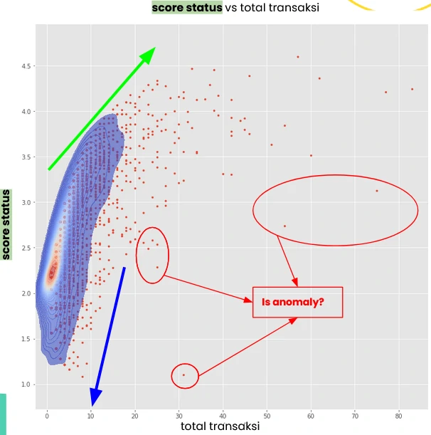
Scores above 3 consistently shift to the right, indicating that strong performance is associated with higher transaction activity (green arrow). In contrast, scores below the 2.23 baseline cluster on the left, reflecting limited engagement. This suggests a clear behavioral pattern: customers who default on their initial transactions are less likely to continue transacting (blue arrow).
That said, the plot also surfaces a subset of outliers. These customers maintain relatively high transaction volumes but still carry low scores, indicating persistent repayment issues despite continued activity. This segment warrants closer attention, as it deviates from the typical relationship between engagement and performance.
Custom Scoring
We can construct a custom scoring model directly from the parameters in the revenue score matrix. One practical formulation is to decompose the score into two components:
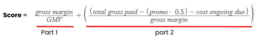
Part 1 (margin efficiency): Theoretical maximum is 1, but in practice it rarely exceeds ~0.5, as gross margin typically does not surpass half of GMV. This component captures how efficiently each transaction converts volume into margin.
Part 2 (cost discipline): This component has a maximum value of 1, representing an ideal state, no over due, related costs, no promotional dependency, and full repayment. The promotion variable is down-weighted with a factor of 0.5, reflecting a partial negative impact rather than treating it as purely detrimental. This coefficient is adjustable depending on business assumptions.
Resulting scale:
Theoretical range: 0 to 2 Practical range: 0 to ~1.5, given the natural constraint on gross margin
This structure ensures the score balances profitability (Part 1) and repayment quality/cost control (Part 2), rather than over-indexing on either dimension.
Data Distribution
From the distribution, the maximum observed score is 0.97, slightly above both the mean (0.95) and median (0.96), indicating a relatively tight concentration of values near the upper bound.
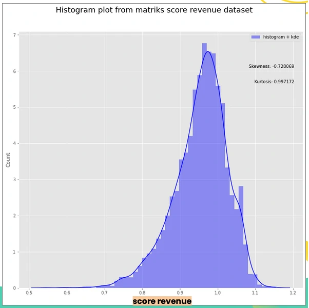
A secondary peak appears around 1.06, suggesting the presence of a distinct subgroup that outperforms the broader population and warrants further investigation.
Overall, the distribution shows a moderate negative skew, with most customers clustering around a score of ~0.5. A large share falls below the 0.97 threshold, indicating weaker revenue performance, typically driven by either higher default-related costs or low transaction activity.
Custom Scoring Result
When plotted as an XY scatter, transaction volume on the x-axis and revenue score on the y-axis, the structure becomes more nuanced.
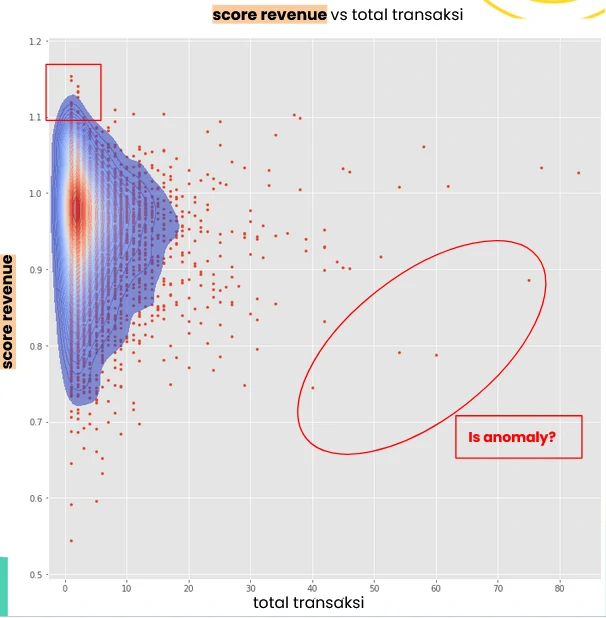
Several patterns emerge:
- Top-end scores (>1.1) are concentrated among customers with low transaction counts (red squares), suggesting strong unit economics but limited scale.
- customers with scores below 1.0 tend to exhibit higher transaction volumes, indicating that increased activity does not necessarily translate into stronger revenue efficiency.
- High-volume customers are largely clustered within the 0.9 to 1.1 range, pointing to a relatively stable but moderate performance band.
- customers with scores below 0.7 show wide variability in activity, most commonly within the 1–10 transaction range, reflecting inconsistent or underperforming behavior.
As with the status score, a subset of anomalous cases stands out—customers who sustain relatively high transaction volumes but generate disproportionately low scores. This segment signals structural inefficiencies, where scale is not converting into profitability and may require targeted intervention.
Combining score status & score revenue
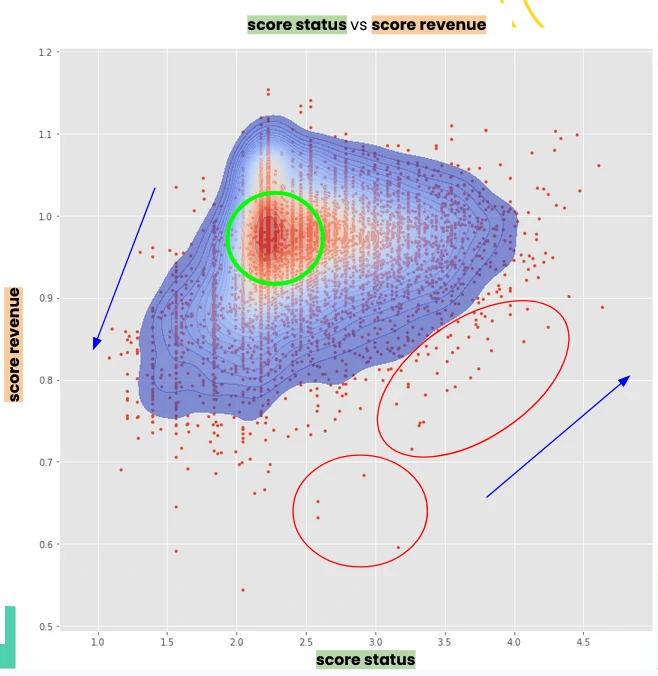
When we plot both scores in a single scatter—status score (y-axis) against revenue score (x-axis)—the overall segmentation becomes clear.
-
Most customers cluster in the mid-performance zone, with revenue scores around 0.9–1.0 and status scores between 2.0 and 2.5. This segment is largely driven by newer customers, whose activity is still building but remains relatively stable.
-
A distinct group sits in the lower-left quadrant, where both revenue and status scores are low. This reflects structurally weak performance, typically driven by a high share of defaulted transactions and the associated cost burden.
-
On the upper end, customers with high status scores generally also exhibit strong revenue scores. The relationship is mutually reinforcing: consistent repayment behavior reduces cost leakage, which improves revenue efficiency, and in turn supports sustained transaction activity that strengthens status.
-
There is, however, a notable exception. A subset of customers (highlighted in the red circle) shows high status scores but comparatively low revenue scores. This pattern suggests mixed transaction quality, likely a combination of performing and defaulted loans, or frequent reliance on promotions, both of which dilute overall profitability despite acceptable repayment behavior.
Proposed Customer Segments
From the combined score distribution, we can define customer segments based on the interaction between revenue and status performance.
Why segmentation instead of fixed categories? Segmentation allows the grouping to adapt to the underlying data distribution, rather than forcing customers into rigid, predefined buckets. As score distributions shift over time, the segment boundaries can be recalibrated accordingly and maintaining relevance and improving decision accuracy.
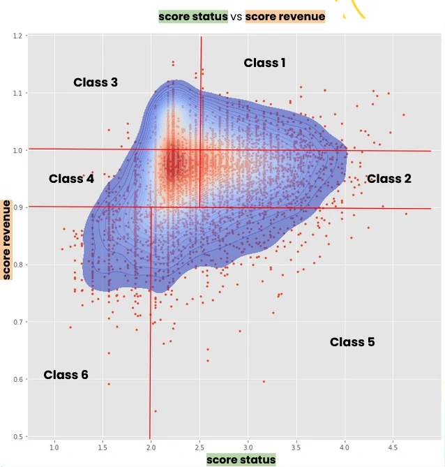
Using the relative position of each customer against the score distribution (low, average, high), we can define at least six actionable segments:
- Class 1 → High status, high revenue
- Class 2 → High status, average revenue
- Class 3 → Low/average status, high revenue
- Class 4 → Low/average status, average revenue
- Class 5 → High status, low revenue
- Class 6 → Low status, low revenue
This segmentation framework is intentionally flexible. Thresholds and group definitions can be adjusted to align with specific business objectives, whether prioritizing risk control, revenue optimization, or customer growth.
So, What next? - Probable Action items
The next step is translating these segments into targeted actions. This should be driven by the specific business objective, whether it’s growth, risk control, or margin optimization.
In example, to sharpen the analysis, we can introduce an additional dimension such as total transaction volume (using marker size or weighting). This makes the distribution within each segment more explicit, highlighting not just performance quality but also scale of activity.
Illustrative Action Direction
We can deepen the analysis by focusing on specific segment behaviors and the gaps between performance dimensions.
-
Class 1 (high status, high revenue) This segment is often composed of customers with strong performance but relatively moderate transaction volume.
Two immediate levers emerge:
- Scale up exposure: assess the feasibility of increasing credit limits to unlock higher transaction throughput.
- Deconstruct success factors: analyze behavioral and operational patterns driving their strong scores, and replicate these conditions across other segments.
This segment represents a controlled growth opportunity. Low risk, high potential upside if volume can be expanded without degrading performance.
- Class 3 (high revenue, low status, low volume) This segment generates strong revenue efficiency but lacks repayment consistency and scale. The priority here is to stabilize credit behavior and improving status without disrupting the underlying profitability.
- Class 5 (high status, low revenue) These customers demonstrate reliable repayment but underperform on revenue. This points to under-monetization, potentially driven by low margins, high promo usage, or suboptimal transaction structure.
- Classes 2 and 5 (strong status, moderate/low revenue) Both segments present a clear opportunity to lift revenue performance while maintaining their already solid repayment profiles, through pricing optimization, reduced promo dependency, or increased transaction value.
Feature Expansion
To better explain score variation, additional variables should be evaluated, such as:
- Commodity type
- Geographic area
- Loan tenor
- Pond count and type
- Other operational or behavioral attributes
These factors can help identify structural drivers behind both revenue and status outcomes.
Integration with RFM Framework
The scoring model can also be reframed within an RFM-like structure:
- F (Frequency) → proxied by status score
- M (Monetary) → proxied by revenue score
- R (Recency) → defined by the latest due date
The choice of due date (instead of order date) is intentional. In a tenor-based system, the most recent meaningful interaction is tied to repayment obligations, not transaction initiation.
Operational Application
These scores can be directly embedded into credit decisioning workflows:
Limit adjustments: calibrate upgrades or downgrades of customer credit limits based on combined score signals Second-layer validation: use the score as an alternative or complementary risk indicator alongside existing models
At an aggregate level, the average or cumulative score per location (point) can serve as a proxy for overall portfolio quality, enabling performance benchmarking and regional strategy alignment.