Real-Time Data Pipeline Using Kafka

data engineering

kafka

• Real-Time Data Pipeline Using Kafka
  • Overview Project
  • Real-Time Object Intelligence Platform
  • Business Impact
  • Data Source
  • Streaming Data Flow Architecture
  • Stream Creation & Real-Time Event Modeling
    • Step 1 — Stream Initialization
    • Step 2 — Event Enrichment via JOIN_EVENTS
    • Step 3 — Spatial Filtering
    • Step 4 — Distance Computation
    • Results
  • Table Creation & Final data
    • Step 1 — Time-Window Aggregation Table
    • Step 2 — Device-Level Latest Event Table
    • Step 3 - Storage Format & Downstream Integration
    • Results
  • Sink to DWH
    • Serialization & Schema Handling
    • Primary Key & Insert Strategy
  • Access by API - Stream Layer (ksqlDB) Endpoints
  • How to install and to use
  • Resource

Overview Project

Imagine having deterministic visibility over any moving asset—whether a vehicle, drone, satellite, wildlife tag, or field team—with precise spatial and temporal resolution. GPS telemetry establishes the foundational signal: exact latitude, longitude, and timestamp. However, geolocation alone only answers where and when. By integrating additional sensors, temperature, acoustic signatures, altitude, vibration, and other environmental parameters, we elevate tracking into contextual intelligence. These multidimensional data streams enable us to infer operational state, behavioral patterns, environmental exposure, and potential anomalies in real time.

To operationalize this capability, we implement a streaming data architecture. Movement behavior is simulated using Brownian motion to realistically model stochastic trajectories, while sensor behavior is generated via parameterized pseudo-random distributions to emulate normal ranges, deviation thresholds, and anomaly rates. Apache Kafka functions as the event backbone for high-throughput ingestion, with ksqlDB enabling real-time joins, windowed aggregations, correlation, and anomaly detection. PostgreSQL serves as the warehouse layer for durable historical storage and state snapshots, while FastAPI exposes low-latency APIs for live and historical access. The result is a unified intelligence system that transforms raw telemetry into actionable insight—supporting fleet optimization, wildlife research, live surveys, expedition safety monitoring, and autonomous vehicle or satellite surveillance.

Real-Time Object Intelligence Platform

Imagine the ability to monitor any moving asset—whether an animal, vehicle, drone, satellite, or fleet unit—with precise spatial and temporal awareness. By embedding GPS trackers, we can capture exactly where an object is and when it was there.

But location is only the baseline.

By integrating additional sensors, temperature, acoustic signals, altitude, vibration, and other environmental parameters, we move beyond tracking into contextual intelligence. These multidimensional signals allow us to understand the real-time condition, behavior, and operational environment of the asset.

System Architecture: To operationalize this, we implement a streaming-first data platform:

1. Apache Kafka: Event backbone for ingesting and orchestrating high-throughput GPS and sensor streams.
2. ksqlDB: Real-time stream processing: joins, time-window aggregations, event correlation, and anomaly detection.
3. PostgreSQL (Data Warehouse layer): Persistent storage for historical records and latest-state snapshots.
4. FastAPI: High-performance API layer for real-time data access from streaming topics or warehouse storage.

Business Impact

This architecture enables continuous tracking, live analytics, and operational decision support in scenarios such as:

1. Fleet management optimization
2. Wildlife behavior research
3. Live survey
4. Expedition, diving and hiking group safety monitoring
5. Drone, unmanned aerial or marine vehicle and satellite operations surveillance

Outcome: A unified, real-time intelligence system that transforms raw movement data into actionable insight.

Data Source

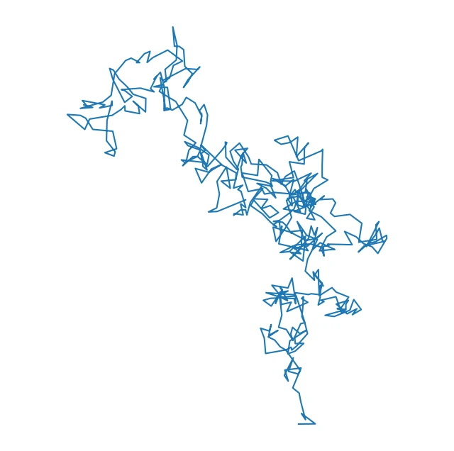
To realistically simulate continuously moving objects with unpredictable trajectories, we will model movement using Brownian motion. This provides a representation of random displacement over time.

For sensor model, we could implements pseudo-random number generators to give random behavior with well-defined parameters such as as normal range, anomaly rate and deviation value.

For this project, The system will be initialized with the following parameters:

1. Longitude = 107
2. Latitude = 9
3. sound range = 30 - 50; anomaly_rate = 25%; deviation = 20%
4. Temperature range = 20 -30; anomaly_rate = 15%; deviation = 20%
5. Altitude range = 1000 - 2000; anomaly_rate = 10%; deviation = 20%

The output of these model can be shown as topics follow:

1. Movement model - Topic: device_location

1. Sensor model - Topic: device_status

Each topics will generate 3 different keys based on 3 devices (dev-1, dev-2, dev-3). To make it more realistic, we separate the message rate for model movement and the sensor model. With:

1. the model movement it produces 1 event / 2 seconds.
2. the sensor model it produces 1 event / 0.5 seconds.

Streaming Data Flow Architecture

The diagram on the right illustrates how streaming data moves from producers to the Data Warehouse layer (in this case, PostgreSQL) and is ultimately served through FastAPI.

Each producer generates event streams with defined event volumes and configurable transmission delays. These events are published into dedicated topics within Kafka, forming the ingestion layer.

ksqlDB acts as the stream processor and first-level consumer:

1. Ingests raw topic data as streams
2. Joins multiple streams into a unified data model
3. Applies time-windowed aggregations (e.g., per device, per interval)
4. Produces enriched and aggregated outputs

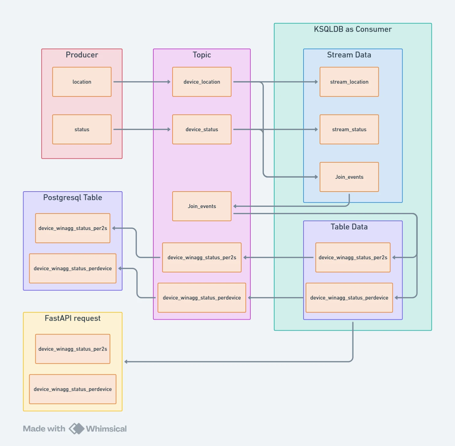
The aggregated results are then persisted into PostgreSQL tables, enabling both historical analysis and latest-state queries.

Finally, FastAPI exposes the data through API endpoints—either directly from ksqlDB for real-time stream queries or from PostgreSQL for structured, persistent analytics.

Result: A scalable, event-driven pipeline that transforms raw streaming events into structured, queryable intelligence.

Stream Creation & Real-Time Event Modeling

Step 1 — Stream Initialization

We establish two primary streams from Apache Kafka topics: stream_location, stream_status

Each stream ingests JSON-formatted events with event_ts defined as the event-time timestamp to ensure accurate temporal processing.

Every record contains:

• id → unique event identifier
• device_id → unique device reference

This structure guarantees event-level traceability and device-level aggregation.

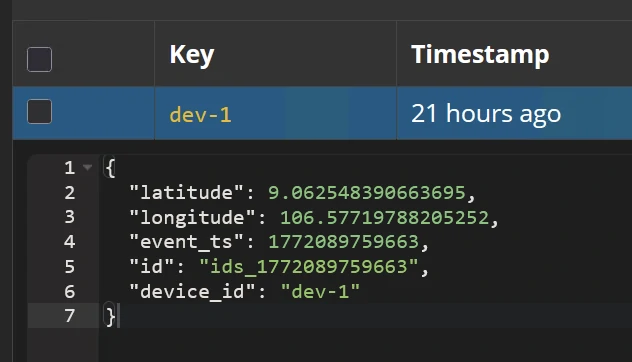
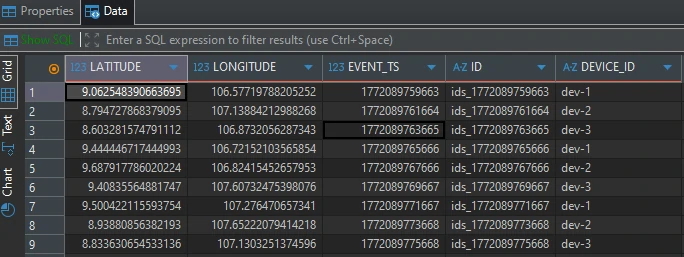
• stream_location

    CREATE STREAM stream_location (
        latitude DOUBLE,
        longitude DOUBLE,
        event_ts BIGINT,
        ID VARCHAR,
        device_id VARCHAR
    ) WITH (
        KAFKA_TOPIC  = 'device_location',
        VALUE_FORMAT = 'JSON',
        TIMESTAMP    = 'event_ts'
    );
  

• stream_status

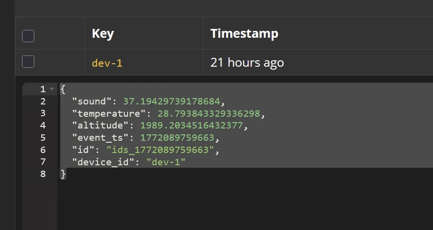
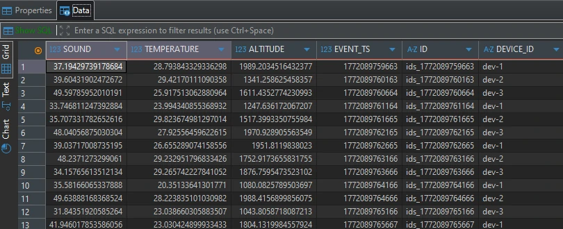
    CREATE STREAM stream_status (
        sound DOUBLE,
        temperature DOUBLE,
        altitude DOUBLE,
        event_ts BIGINT,
        ID VARCHAR,
        device_id VARCHAR
    ) WITH (
        KAFKA_TOPIC  = 'device_status',
        VALUE_FORMAT = 'JSON',
        TIMESTAMP    = 'event_ts'
    );
  

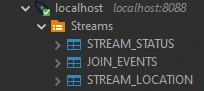
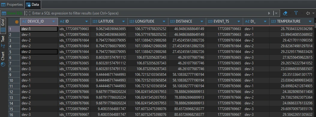
Step 2 — Event Enrichment via JOIN_EVENTS

We implement a stream-joining process (JOIN_EVENTS) using ksqlDB to construct a unified event model.

Join Strategy

• Left Join: stream_location → stream_status. Location acts as the primary reference (baseline signal).
• Temporal Constraint: LEFT JOIN WITHIN 2 SECONDS ON device_id

For each location event:

• If a status event from the same device occurs within ±2 seconds → it is attached
• If no match is found → the location event is retained

This ensures spatial continuity even when status telemetry is intermittent or generate more data compare to spatial data.

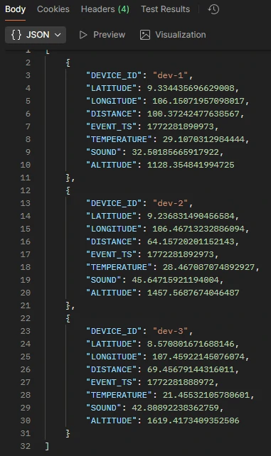
• JOIN_EVENTS

    CREATE STREAM JOIN_EVENTS AS
    SELECT
        SL.ID ID,
        SL.DEVICE_ID DEVICE_ID,
        SL.LATITUDE,
        SL.LONGITUDE,
        GEO_DISTANCE(SL.LATITUDE, SL.LONGITUDE, 9.0, 107.0) DISTANCE,
        SL.EVENT_TS EVENT_TS,
  
        SS.DEVICE_ID as DI_,
        SS.temperature,
        SS.sound,
        SS.altitude
    FROM STREAM_LOCATION AS SL
    LEFT JOIN STREAM_STATUS AS SS
        WITHIN 2 SECONDS
        ON SL.DEVICE_ID = SS.DEVICE_ID
    WHERE
        1=1
        and SL.LATITUDE BETWEEN 8 AND 10
        and SL.LONGITUDE BETWEEN 106 AND 108
    EMIT CHANGES;
  

Step 3 — Spatial Filtering

We constrain the operational boundary:

• Longitude : 106 – 108
• Latitude : 8 – 10

Events outside this geofence are excluded to maintain geographic relevance and reduce processing noise.

Step 4 — Distance Computation

Using GEO_DISTANCE, we calculate the great-circle distance between each device coordinate and a fixed reference point: Reference location:

• Longitude = 107.0
• Latitude = 9.0

The function computes spherical distance (decimal degrees input) and returns results in kilometers (KM).

Results

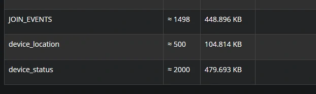
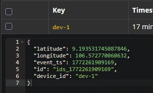
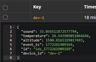
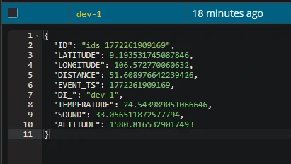
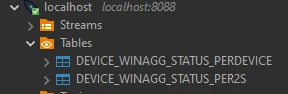
Table Creation & Final data

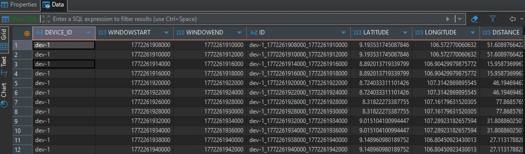
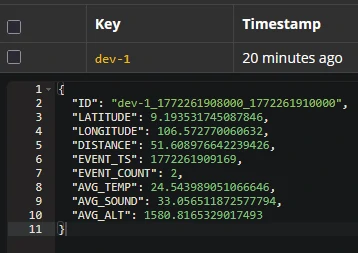
Step 1 — Time-Window Aggregation Table

We first construct a time-aggregated table using ksqlDB, designed to normalize high-frequency sensor events that may arrive at different intervals per device. The objective is to transform raw telemetry into structured, time-bucketed metrics per device.

Within each defined time window, we compute:

• Average values for core sensor parameters
• Maximum event_ts to retain the latest timestamp within the window

• Event count to quantify data density per interval

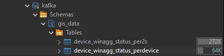
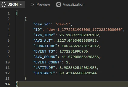
• device_winagg_status_per2s

    CREATE TABLE device_winagg_status_per2s
    WITH (
        KEY_FORMAT   = 'AVRO',
        VALUE_FORMAT = 'AVRO'
    ) AS
    SELECT
        CONCAT( CAST(DEVICE_ID AS STRING), '_', CAST(WINDOWSTART AS STRING), '_', CAST(WINDOWEND AS STRING)) AS ID,
        DEVICE_ID,
        AS_VALUE(DEVICE_ID) as "dev_id",
        AVG(LATITUDE) LATITUDE,
        AVG(LONGITUDE) LONGITUDE,
        AVG(DISTANCE) DISTANCE,
  
        MAX(EVENT_TS) EVENT_TS,
        COUNT(*) AS event_count,
        AVG(TEMPERATURE) as avg_temp,
        AVG(SOUND) as avg_sound,
        AVG(ALTITUDE) as avg_alt
    FROM JOIN_EVENTS
    WINDOW TUMBLING (SIZE 2 SECONDS)
    GROUP BY DEVICE_ID
    EMIT CHANGES;
  

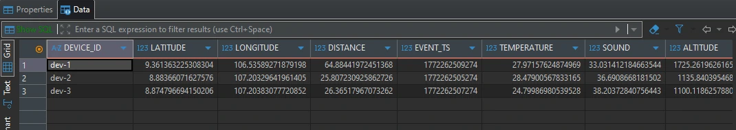
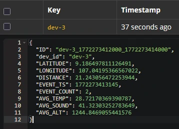
Step 2 — Device-Level Latest Event Table

Next, we create a second aggregation layer that captures only the most recent event per device.

For every device, this table returns the most recent value metrics from the offset data.

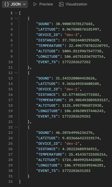
• device_winagg_status_perdevice

    CREATE TABLE device_winagg_status_perdevice
    WITH (
        KEY_FORMAT   = 'AVRO',
        VALUE_FORMAT = 'AVRO'
    ) AS
    SELECT
        DEVICE_ID,
        LATEST_BY_OFFSET(LATITUDE) AS LATITUDE,
        LATEST_BY_OFFSET(LONGITUDE) AS LONGITUDE,
        LATEST_BY_OFFSET(DISTANCE) AS DISTANCE,
        LATEST_BY_OFFSET(EVENT_TS) AS EVENT_TS,
        LATEST_BY_OFFSET(TEMPERATURE) AS TEMPERATURE,
        LATEST_BY_OFFSET(SOUND) AS SOUND,
        LATEST_BY_OFFSET(ALTITUDE) AS ALTITUDE
    FROM JOIN_EVENTS
    GROUP BY DEVICE_ID
    EMIT CHANGES;
  

Step 3 - Storage Format & Downstream Integration

Both tables are serialized in AVRO format, ensuring schema consistency and seamless sinking into the Data Warehouse layer (e.g., PostgreSQL).

Results

Sink to DWH

To store streaming results into the Data Warehouse layer (e.g., PostgreSQL), we utilize the Kafka Connect JDBC Sink Connector. This enables direct ingestion of Kafka topics into relational tables with schema enforcement.

Serialization & Schema Handling

Since events are serialized in AVRO format, we configure:

• value.converter = io.confluent.connect.avro.AvroConverter
• key.converter = io.confluent.connect.avro.AvroConverter

This ensures schema-aware deserialization and compatibility with PostgreSQL table structures.

Primary Key & Insert Strategy

We apply different persistence strategies aligned with analytical purpose:

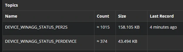
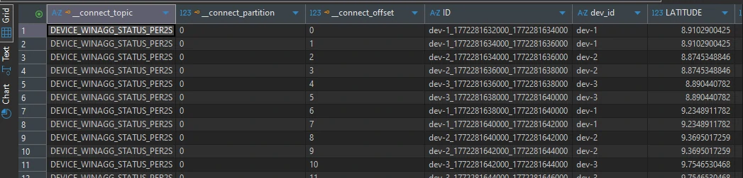
• DEVICE_WINAGG_STATUS_PER2S
  • pk.mode = kafka
  • insert.mode = insert

  

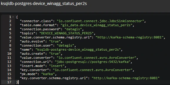
  Each record is uniquely identified using Kafka metadata (topic, partition, offset). Result: Every aggregation window generates a new immutable row—ideal for historical analysis.

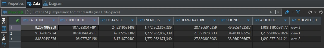
• DEVICE_WINAGG_STATUS_PERDEVICE
  • pk.mode = record_key
  • insert.mode = upsert

  

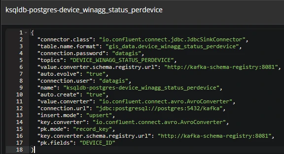
  Records are keyed by device identifier. Result: Each incoming event updates the existing device row, maintaining a real-time “latest state” table.

Access by API - Stream Layer (ksqlDB) Endpoints

The system exposes unified API endpoints via FastAPI, enabling data retrieval from both the streaming layer ksqlDB (Low-latency stream queries) and the warehouse layer PostgreSQL (Structured historical queries).

• /stream/raw
  • Accesses: DEVICE_WINAGG_STATUS_PER2S
  • Purpose: Retrieve time-windowed (2-second) aggregated data
  • Query Parameters:
    • device_id → default: dev-1
    • limit → default: 10

    

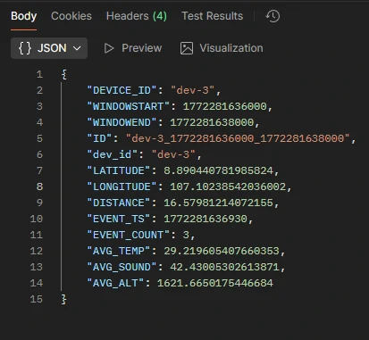
• /stream/latest
  • Accesses: DEVICE_WINAGG_STATUS_PERDEVICE

  • Purpose: Retrieve the latest aggregated snapshot per device

    

• /stream/postgresql/raw
  • Accesses: DEVICE_WINAGG_STATUS_PER2S
  • Purpose: Retrieve persisted 2-second aggregation records
  • Query Parameters:
    • device_id → default: dev-1
    • limit → default: 10

    

• /stream/postgresql/latest
  • Accesses: DEVICE_WINAGG_STATUS_PERDEVICE

  • Purpose: Retrieve the latest stored device state from the warehouse

    

How to install and to use

1. install kafka containers

   docker compose --profile kafka up -d

2. install postgresql container

   docker-compose up -d --build postgres

3. access the container with

   docker exec -it ksqldb-server ksql

   docker exec -it etl_kafka sh

4. run the generator

   python producer_device_status.py

   python producer_device_location.py

5. run the FastAPI with

   uvicorn main:app --host 0.0.0.0 --port 8080 --reload

Resource

• https://github.com/imanursar/kafka_exp
• Slides