A/B Testing 101
Solutions
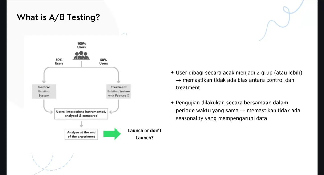
What Is A/B Testing?
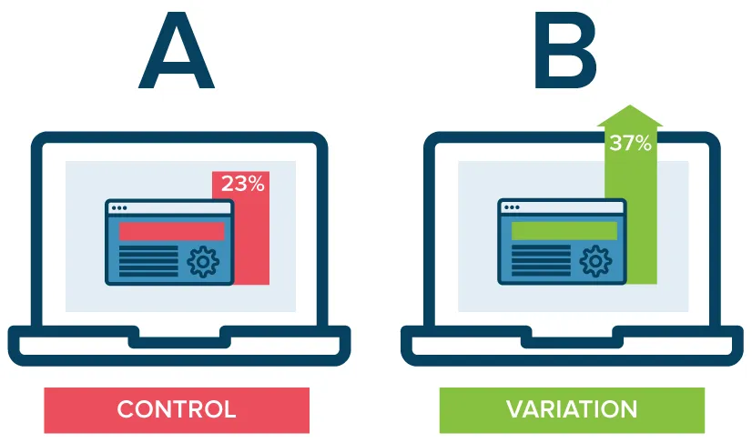
- AB testing (also known as split testing or bucket testing) compares two versions of a thing against each other to determine which one performs better.
- AB testing is essentially an experiment where two or more variants of a thing are shown to users at random. Statistical analysis is used to determine which variation performs better for a given conversion goal.
- Use AB test to determine whether the effect you observed is significant statistically and practically.
Why is it so important?
- With A/B testing, it can increase customer satisfaction with small changes without changing all things.
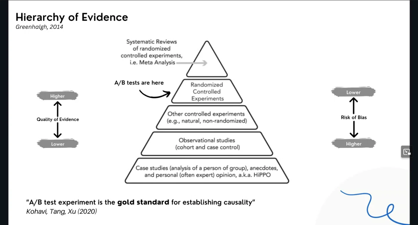
- Hierarchy of evidence
- Measuring impact from an action.
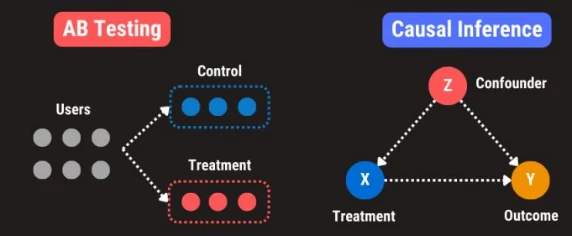
AB Testing vs Causal Inference
- AB testing: Detect effect in a randomized controlled trials
- Causal inference: Measure effect in naturalistic observation
| Comparison | AB Testing | Causal Inference |
|---|---|---|
| Use Cases | Minor UI Tweaks (e.g. Color), Online Ads optimization | Optional treatment or feature, Offline Ads performance |
| Randomization | Random assignment | Self-selection; observational study |
| Experiment Duration | Short-Term; 1 to 2 weeks | Long-Term; 1 to 3 Months |
| Statistical Method | T-Test, Z-Test, Mann Whitney U-Test | PSM, DID, RDD, Synthetic Controls |
| Limitations | Limits the test to a single variable | Difficult to establish causality in non-experimental settings |
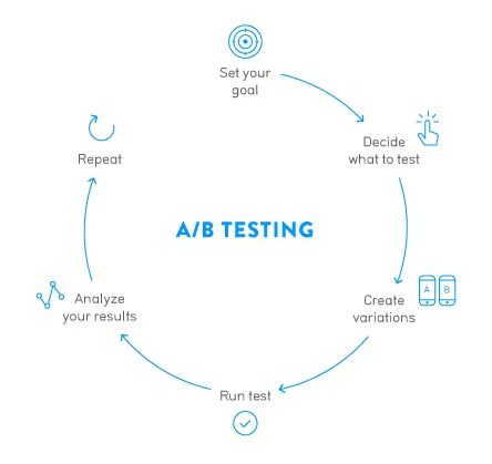
Workflow
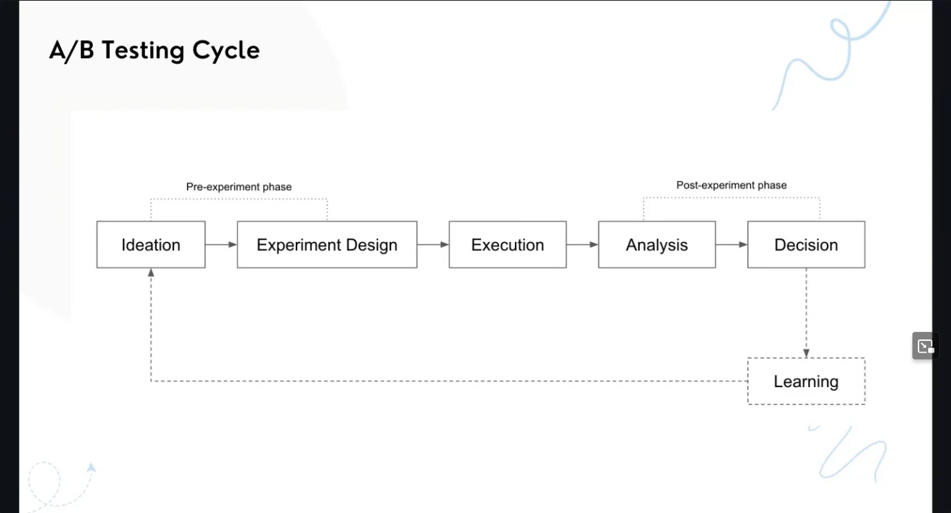
AB Testing Cheatsheet
- Hypothesis Statements
- Business Hypothesis: We expect a metric to noticeably decline/stay neural/increase.
- Statistical Hypothesis
- Ho: No change on KPI
- Ha: Change on KPI
- Experiment Parameters
- Significance Level: α= 0.01 to 0.10
- Practical Significance: ▲ >= 0.1% to 10%
- Statistical Power: Power = 80 to 95%
- Sample Size Calculation
- Experiment Duration: 1 to 4 weeks
- Randomization: User, device, geo
-
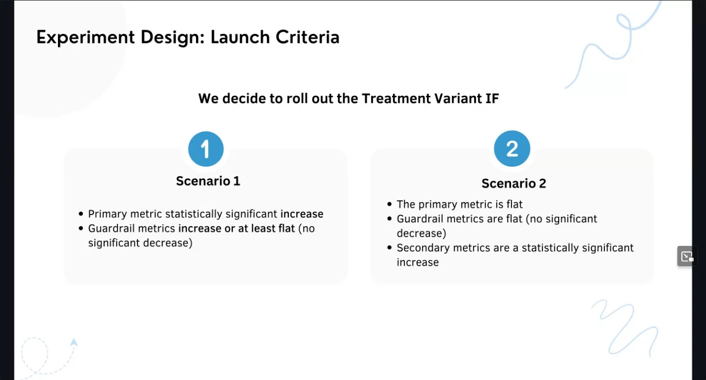
Launch Decision
P-Value Metric Outcome Decision 0.02 Significant Increase Launch 0.08 Significant Increase Launch with caution 0.08 Not Significant Increase Run experiment longer 0.08 Not Significant Increase Run experiment longer 0.08 Significant Decrease Do not launch 0.02 Significant Decrease Do not launch - Violation Checks
- SUTVA
- Novelty Effect
- Change Aversion
- Holiday Effect
- Sample Ratio Mismatch
- Instrumentation Effect
- Survivorship Bias
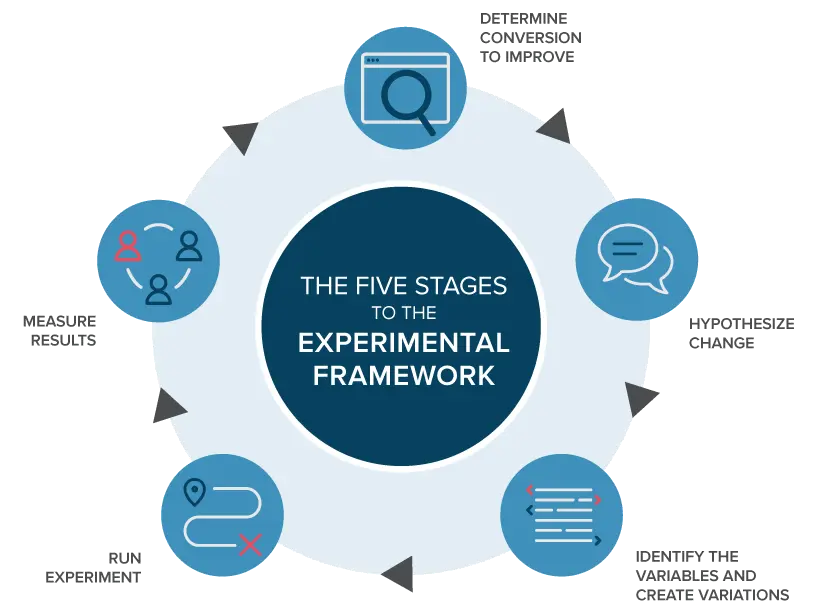
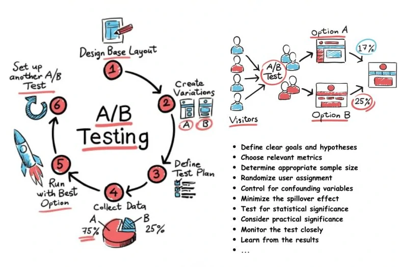
How to Perform an A/B Test?
- Define metrics
| Metric type | Metric name | Reason |
|---|---|---|
| primary metrics → metrik utama yang menentukan kesuksesan eksperimen | conversion | rate up |
| Guardrail metrics → metriks yang tidak boleh turun | revenue | stable |
| secondary metrics → metriks penunjang yang digunakan sebagai supporting metrics | Click-through rate | if this down, the primary should be down |
- Define how many variant
- Define power analysis: Define the sample size and experiment duration.
- Data Collection: We need to collect enough data to concentrate on the target problem.
- Split data in half for conversion target. (We usually say control and test group) Target variables can be one of them: a headline, a button, an image, or color used for design.
- Formulate Hypothesis: We have the current variation. We want to create hypothesis-based variation. This variation is another version of your current version with changes that you want to test.
- Run Test: Once you have a hypothesis ready, test it against various parameters like how much confidence you have of it winning, its impact on macro goals, and how easy it is to set up, and so on.
- Results Analyzing: Test results are scored.
- Launch criteria
What is Hypothesis Testing?
- Start with the existing version of the tested element within it. That existing version is now termed the “baseline” (or variation A).
- Set up the alternative variation, the “treatment” (or variation B).
- Calculate the required sample size. This calculation is based on the baseline’s current conversion rate (which must be already known), the minimum difference in performance you wish to detect, and the desired Statistical Power.
Statistic method
- Shapiro-Wilks Test for both group
- Levene’s Test for Homogeneity of variances
- t-test for comparing groups.
- Minimum Detectable Effect (MDE) - minimum uplift yang ingin terukur
- Chi-Square Test
Error
- False positive - The data from the test indicates a meaningful difference between the control and treatment experiences, but in truth there is no difference.
- False negative - The data do not indicate a meaningful difference between treatment and control, but in truth there is a difference.
- False positives and statistical significance
- By convention, this false positive rate is usually set to 5%: for tests where there is not a meaningful difference between treatment and control, we’ll falsely conclude that there is a “statistically significant” difference 5% of the time. Tests that are conducted with this 5% false positive rate are said to be run at the 5% significance level.
- The false positive rate is closely associated with the “statistical significance” of the observed difference in metric values between the treatment and control groups, which we measure using the p-value.
P-value
- Decide null hypothesis
- Calculate possible outcomes and their associated probabilities
- Compare this probability distribution of outcomes to the data we’ve collected.
- Count up the probabilities associated with every outcome that is less likely than our observation.
- Measure the probability of seeing a result as extreme as our observation, if the null hypothesis were true.
- the P-value is a sum up the probabilities (to the agree with null hypothesis or against it.
- The interpretation is as follows: were we to repeat, many times, the experiment in p-value% of those experiments the outcome would feature at least prob %.
- material
Repeated significance testing errors
- Assuming there is no underlying difference between A and B, how often will we see a difference like we do in the data just by chance? The answer to that question is called the significance level, and “statistically significant results” mean that the significance level is low, e.g. 5% or 1%.
- However, the significance calculation makes a critical assumption that you have probably violated without even realizing it: that the sample size was fixed in advance. If instead of deciding ahead of time, “this experiment will collect exactly 1,000 observations,” you say, “we’ll run it until we see a significant difference,” all the reported significance levels become meaningless. This result is completely counterintuitive and all the A/B testing packages out there ignore it.
- The problem will be present if you ever find yourself “peeking” at the data and stopping an experiment that seems to be giving a significant result. The more you peek, the more your significance levels will be off.
- What can be done?
- the best way to avoid repeated significance testing errors is to not test significance repeatedly. Decide on a sample size in advance and wait until the experiment is over before you start believing the “chance of beating original” figures that the A/B testing software gives you.
- “Peeking” at the data is OK as long as you can restrain yourself from stopping an experiment before it has run its course.
- Don’t report significance levels until an experiment is over, and stop using significance levels to decide whether an experiment should stop or continue.
Sample Size

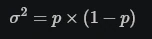
- Where δ is the minimum effect you wish to detect and σ2 is the sample variance you expect. if it’s just a binomial proportion you’re calculating (e.g. a percent conversion rate) the variance is given by:
- Report how large of an effect can be detected given the current sample size.
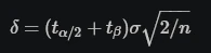
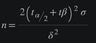
- Where the two t’s are the t-statistics for a given significance level α/2 and power (1−β).
- Statistical power 1−β = Percent of the time the minimum effect size will be detected, assuming it exists. (80%)
- Significance level α = Percent of the time a difference will be detected, assuming one does NOT exist. (5%)
Details
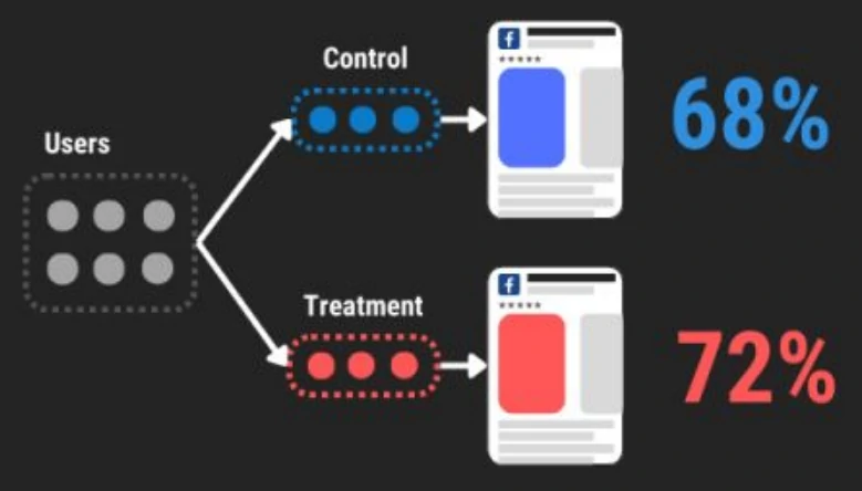
- Splitting data
- We run an A/B test by splitting our customers into two groups: the A group acts as a control and gets the standard price. In contrast, the B group gets the price discount.
- Crucially, to avoid selection biases we choose our groups randomly, so that when we compare the average profits across groups, we can rest assured that we in fact estimated the causal effect.
- Formulate Hypothesis
- All experiments begin with a hypothesis: a guess about behavioral change that will result from some alteration to a product, process, or message. The change might be to a user interface, a new user on boarding flow, an algorithm that powers recommendations, marketing messaging or timing, or any number of other areas. If the organization built it or has control over it, it can be experimented on, at least in theory.
- Hypotheses are often driven by other data analysis work. For example, we might find that a high percentage of people drop out of the checkout flow, and we could hypothesize that more people might complete the checkout process if the number of steps were reduced.
- Success Metric
- The second element necessary for any experiment is a success metric. The behavioral change we hypothesize might be related to form completion, purchase conversion, click-through, retention, engagement, or any other behavior that is important to the organization’s mission. The success metric should quantify this behavior, be reasonably easy to measure, and be sensitive enough to detect a change. Click-through, checkout completion, and time to complete a process are often good success metrics. Retention and customer satisfaction are often less suitable success metrics, despite being very important, because they are frequently influenced by many factors beyond what is being tested in any individual experiment and thus are less sensitive to the changes we’d like to test. Good success metrics are often ones that you already track as part of understanding company or organizational health.
- Randomly Assigns
- The third element of experimentation is a system that randomly assigns entities to a control or experiment variant group and alters the experience accordingly. This type of system is also sometimes called a cohorting system.
- Because we create our control (“A”) and treatment (“B”) groups using random assignment, we can ensure that individuals in the two groups are, on average, balanced on all dimensions that may be meaningful to the test. Random assignment ensures, for example, that the average length of Netflix membership is not markedly different between the control and treatment groups, nor are content preferences, primary language selections, and so forth. The only remaining difference between the groups is the new experience we are testing, ensuring our estimate of the impact of the new experience is not biased in any way.
- Time process
- Relative base on the business with common time in 2 weeks or 1 month.
- It depends on the power of the test we want to have. Typically, we choose 80% as the threshold. Statistical power is the probability that a test rejects a false null hypothesis. Why 80%? I have no idea. It looks like some tradition or “best practice.” Is it enough? We are not trying to discover a cure for cancer, so I assume 80% is enough.
- The required number of samples -
- To calculate the required number of samples we need to define three parameters.
- Statistical power defined (80%)
- Significance level - We need it to decide whether the null hypothesis should be rejected and also to calculate the number of samples. We are going to use a standard value too (5%).
- The effect size - The value describes the difference in terms of the number of standard deviations that the means are different. This value is the minimal difference we want to detect by the A/B test.
- To calculate the required number of samples we need to define three parameters.
The broad lesson is that there is always something we won’t be able to control.
Pitfall and Remedy
- Mistake novelty effect as real effect
- Novelty effect is when customers engage with a new feature simply because it’s new, but not because they like it. You might see the treatment gets more engagement than control in the beginning, but it’s not the real effect.
- Remedy: Instead of analyzing all customers with the same cut-off for start time and end time, do a cohort analysis based on when customers get assigned to the treatment group, and see whether this effect wears off with time.
- Cannibalization
- The treatment you test might have a positive impact for your experiment, but it might hurt other features on the website, and that’s why it’s call ‘cannibalization’. But sometimes the effect is hard to measure.
- Remedy: use linear models to estimate interaction effect. You can create four cohorts and analyze them: the cohort that are in controls for both experiments, the cohort that in treatments for both experiments, and also isolate the cohorts that are only in one experiment. You need to make sure the cohorts have similar duration of exposure to compare. Try to understand the entire customer journey, top priority business metrics to optimize for, instead of just focusing on the performance of your experiment. Understand the ecosystem of where your feature lives in.
- “Cherry-pick” metrics for launch decisions
- Sometimes decision makers really want to launch a feature, and they would pick whatever looks positive to support their decisions, which violates the principals of statistical testing.
- Remedy: have no more than three core metrics, and have 1-2 secondary metrics to make decisions. The key is to decide on those metrics BEFORE you start experimentation, and stick to them. Don’t move the goal posts just because you want to launch it. If you see something interesting, investigate it, treat it as a new assumption, and don’t make your decision based on an unexpected change.
Report
- Result’s Significance Status - Does the variant perform significantly better/worst than the control?
- Comparing the distribution statistics value with the distribution table value. We get a significant result when the distribution statistics value is greater than the table value.
- Comparing the obtained p-value with the significance level threshold (alpha). p-value is as small as possible since we would get a significant result when the p-value is smaller than alpha.
- Metrics’ Delta Confidence Interval
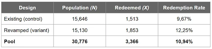
- Report the lift’s exact magnitude by subtracting the revamped design’s redemption rate from the existing one’s. we get a lift (delta) of 12.25%-9.67%=2.58%.
- The confidence interval calculation. example data:
- The steps are as follows:
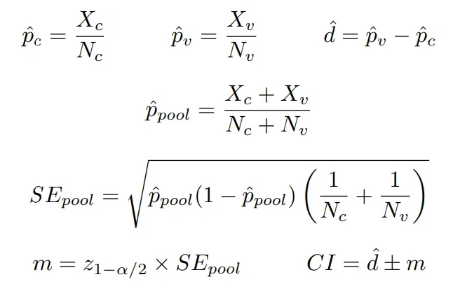
- Compute observed redemption rate in the control group (p_c hat)
- Compute observed redemption rate in the variant group (p_v hat)
- Compute the center of confidence interval (d hat). This is the ‘delta’ between p_v hat and p_c hat
- Compute observed pooled redemption rate (p_pool hat)
- Use p_pool hat, control population size, and variant population size to compute the pooled standard error (SE_pool)
- Compute the deviation of the confidence interval (m). Recall that we use alpha =5% (i.e., z value at cumulative probability 0.975 is 1.96)
- Finally, compute our confidence interval (CI)!
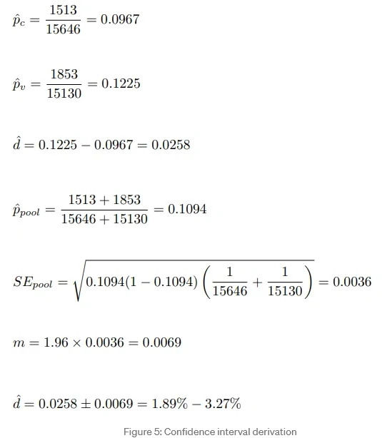
- We got a confidence interval of 1.89% — 3.27%. This means we expect 95% of the time that the delta between the revamped design’s redemption rate and the existing one’s would lie within the 1.89% — 3.27% range.
- Layman terms, we are quite confident that we would get a metrics lift of 1.89% — 3.27% if we roll out the revamped design into production. Much better information than simply saying a single number of 2.58% lift.
- This reads we are 95% sure that the variant group would gain around 1.89% — 3.27% lift over the control.
- Experiment’s Statistical Power
- Statistical power: is the ability of the experiment to detect an effect (metrics difference) that is actually present in reality (the ground truth).
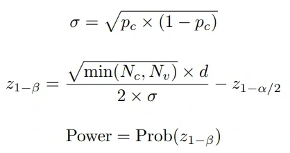
- the minimum detectable effect value (denoted by d): It is the threshold of metrics change/lift that we consider meaningful to be detected robustly in the experiment. Suppose in this experiment we only care of a change of at least 1% in the redemption rate, then we have d = 1%.
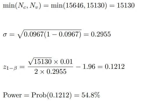
- Z-score:
- The power of our experiment is 54.8%, which means the likelihood is 54.8% for the experiment to be able to detect a non-zero effect (i.e., redemption rates between variant and control is different) if there is truly an effect (i.e., redemption rates between variant and control is truly different — as the ground truth).
-
the rule of thumb for a good experiment is having a power of 80%
- Another interpretation of 54.8% power is there is a probability of 45.2% (100%-54.8%) that the experiment cannot conclude that there is a non-zero effect between control and variant, although the effect does present in reality.
- Example
- The result is significant, i.e., there is enough evidence to state that there is a significant difference in redemption rates obtained by the two designs.
- The metrics’ delta confidence interval is 1.89% — 3.27%, meaning we would get a metrics lift of 1.89% — 3.27% if we roll out the revamped design into production (i.e., we win the variant group).
- The statistical power of the experiment is 54.8%. That is, the likelihood is 54.8% for the experiment to detect a non-zero effect (i.e., redemption rates between variant and control is different) if there is truly an effect in reality.