Pgvector - 101

Vector Database

Postgresql

• Pgvector - 101
  • What is pgvector
  • Installation
  • Enabling the extension
  • Verify the extension
  • Check available operators
  • Creating a Table with a Vector Column
  • Create index for faster similarity search (HNSW - recommended)
  • Insert the data
  • Running a query
  • Choosing a Distance Metric
  • Indexing
  • HNSW Index
  • IVFFLAT Index
  • Filtering

What is pgvector

pgvector is an open-source PostgreSQL extension that adds native vector search to your existing database. Rather than moving your embeddings to a dedicated vector store, pgvector keeps them alongside your relational data, preserving PostgreSQL’s transactional guarantees, JOIN semantics, point-in-time recovery, and the full SQL query language.

This extension adds:

1. Vector data type for storing embeddings.
2. SQL distance operators for ordering query results by similarity.
3. Two index types — HNSW and IVFFlat — for accelerating nearest-neighbor lookups at scale.

Installation

1. For linux: sudo apt install postgresql-18-pgvector
2. For Windows: Installation for Windows

Enabling the extension

  CREATE EXTENSION IF NOT EXISTS vector;

Verify the extension

  SELECT * FROM pg_extension WHERE extname = 'vector';

Check available operators

  SELECT
    opfname AS operator_family,
    opcname AS operator_class
  FROM pg_opclass
  WHERE opcname LIKE 'vector%';

Creating a Table with a Vector Column

  DROP TABLE IF EXISTS products;
  CREATE TABLE products (
    id          SERIAL PRIMARY KEY,
    name        TEXT NOT NULL,
    category    TEXT,
    description TEXT,
    metadata    JSONB DEFAULT '{}',
    price       NUMERIC(8,2),
    embedding   vector(1536),
    create_at   TIMESTAMP DEFAULT NOW()
  );

The vector(1536) column holds one embedding per row. That number must match the output dimension of your model; adjust it accordingly if you use a different one.

Create index for faster similarity search (HNSW - recommended)

    CREATE INDEX ON products
    USING hnsw (embedding vector_cosine_ops);

Insert the data

  INSERT INTO products (name, category, description, embedding) VALUES
  ('Merrell Moab 3 GTX',      'Footwear',  'Waterproof hiking boot for all-day trail comfort',        '[0.82, 0.15, 0.44]'),
  ('Salomon Speedcross 6',    'Footwear',  'Aggressive trail runner for muddy and technical terrain', '[0.79, 0.21, 0.38]'),
  ('Black Diamond Spot 400',  'Lighting',  'Rechargeable headlamp with 400 lumens and waterproofing', '[0.11, 0.88, 0.22]'),
  ('Petzl ACTIK CORE',        'Lighting',  'Lightweight headlamp for hiking and camping',             '[0.09, 0.91, 0.19]'),
  ('Osprey Atmos AG 65',      'Backpacks', 'Anti-gravity backpack for multi-day backcountry trips',   '[0.55, 0.30, 0.77]'),
  ('Gregory Baltoro 75',      'Backpacks', 'High-volume pack for extended wilderness expeditions',    '[0.58, 0.28, 0.81]');

Running a query

  SELECT
    name,
    category,
    description,
    embedding <-> '[0.80, 0.19, 0.40]' AS distance,
    1 - (embedding <-> '[0.80, 0.19, 0.40]') AS similarity,
    (embedding <-> '[0.80, 0.19, 0.40]') * -1 AS similarity_inner_prod,
  FROM products
  ORDER BY distance -- smallest first = most similar
  LIMIT 3;

Choosing a Distance Metric

Common metrics (ordered by how it used):

• L2 distance treats vectors as points in space and measures the geometric distance between them. It works best when vector magnitude carries meaningful information.
• Cosine distance is 1 - cosine similarity and measures the angle between vectors rather than their length. This makes it the preferred choice for text embeddings generated by language models.
• Inner product is useful in recommendation systems, where embeddings are trained so that dot products directly represent similarity. pgvector returns the negative inner product, so you should negate the result to get the actual similarity score.
• L1 distance weights each dimension equally without squaring the differences, giving it mild robustness to outliers compared to L2.
• Hamming and Jaccard apply only to binary vectors, used for memory-efficient quantized representations.

Most LLM-based embedding APIs produce normalized or near-normalized vectors, where semantic meaning is encoded in direction, not magnitude. Because of this, cosine distance generally delivers more accurate semantic rankings for search and retrieval workloads.

Indexing

Without an index, every similarity query performs a full sequential scan: PostgreSQL computes the distance between the query vector and every row in the table. That is acceptable at ten thousand rows. At a million rows, query latency becomes a serious problem.

Index types on pgvector:

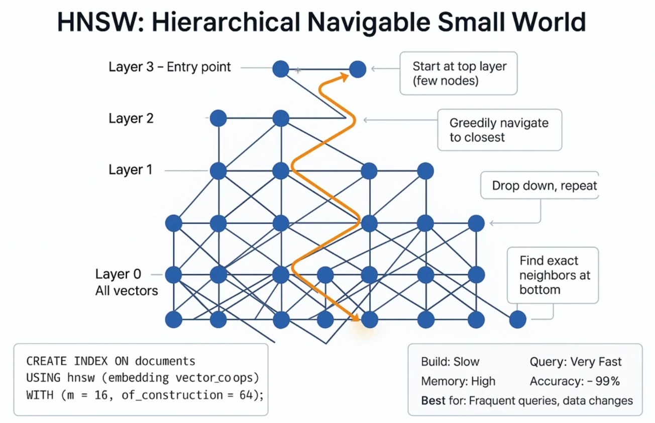
• Hierarchical Navigable Small Worlds (HNSW) constructs a multi-layer graph where each node connects to a bounded number of neighbors across multiple levels of resolution. HNSW gives the best speed-to-recall ratio of the two options, but constructing the graph requires more memory and takes longer than IVFFlat.
  • Fast queries
  • More memory
  • Handles updates
  • default setting

  

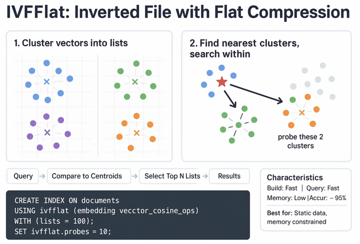
• Inverted File Flat (IVFFlat) partitions the vector space into a fixed number of clusters during index construction, then at query time searches only the clusters closest to the query vector. It builds faster and uses less memory, but those cluster boundaries are fixed at build time.
  • Fast build
  • Less memory
  • Static data
  • Less cost

  

• Comparison

  • 

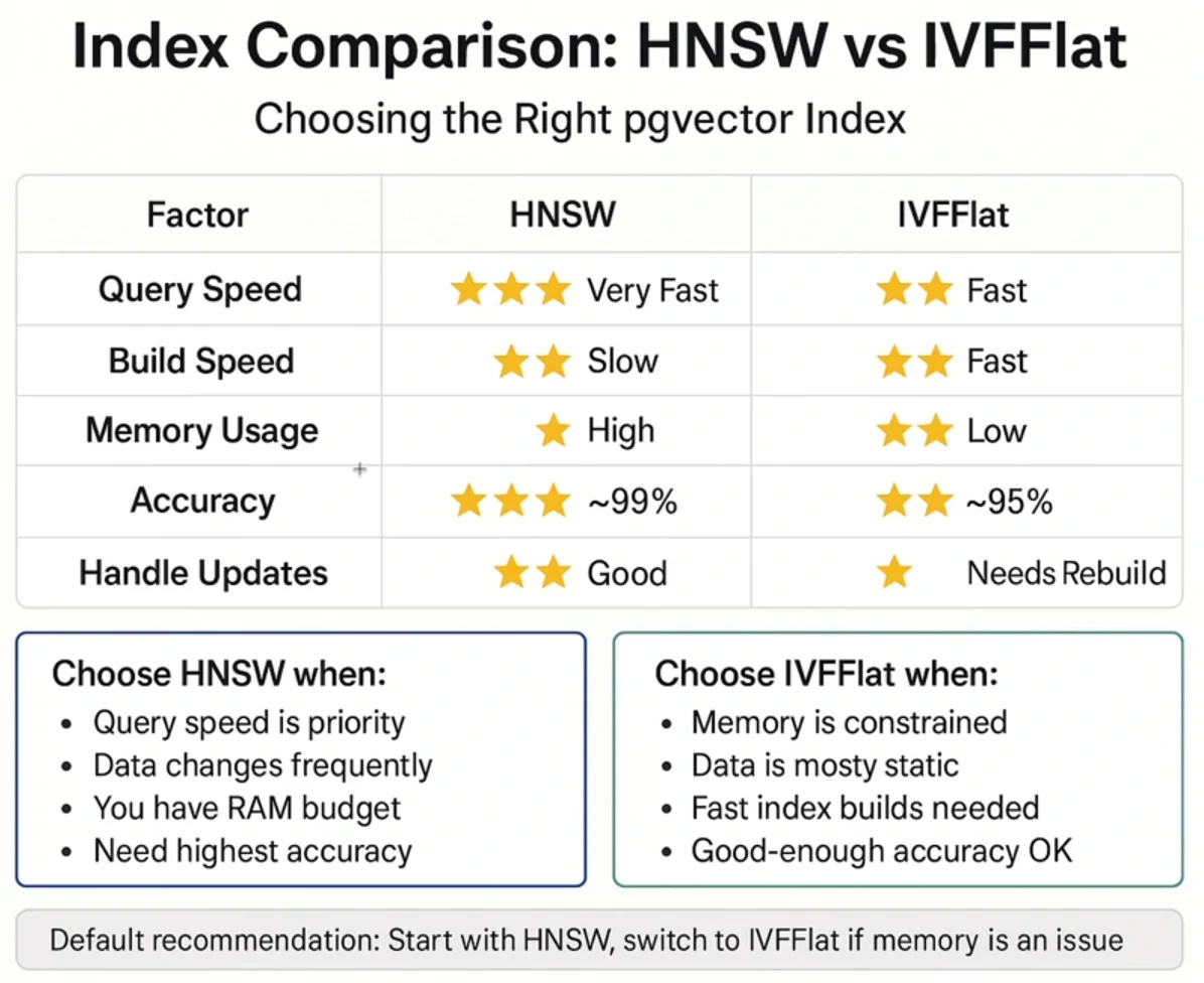
The operator class in your index must match the distance operator in your queries. Always verify with EXPLAIN that the index is being used when needed.

HNSW Index

• Adding an hnsw Index

  CREATE INDEX products_hnsw_idx ON products
  USING hnsw (embedding vector_cosine_ops)
  WITH (m = 16, ef_construction = 64);
  

  where:

  • m = the maximum connections per node in the graph.
    • low (8-16): smaller index, faster builds.
    • high (32-64): larger index, higher accuracy.
  • ef_construction = controls the size of the candidate list during graph construction. with good default = 40.
    • low (32-64): Faster search
    • high (200+): higher accuracy

• Check index size

  SELECT
      indexname,
      pg_size_pretty(pg_relation_size(indexname::regclass)) AS size
  FROM pg_indexes
  WHERE tablename = 'documents';
  

• Set search parameter

  -- Higher = more accurate but slower
  SET hnsw.ef_search = 100;
  

• Verify index

  EXPLAIN ANALYZE
  SELECT content
  FROM documents
  ORDER BY embedding <=> (
    SELECT array_agg(random())::vector(1536) 
    FROM generate_series(1, 1536)
  )
  LIMIT 5;
  

IVFFLAT Index

• Create IVFFlat index. lists = number of clusters (rule: sqrt(rows) to rows/1000). For 1M rows: lists = 1000.

  -- First, check how many rows you have
  SELECT COUNT(*) FROM documents;
  

• Create index with appropriate lists value
  • For small datasets (< 1000 rows) - WITH (lists = 10)
  • For medium datasets (1000-100K rows) - WITH (lists = 100)
  • For large datasets (100K-10M rows) - WITH (lists = 1000)

  CREATE INDEX documents_embedding_ivfflat_idx ON documents
  USING ivfflat (embedding vector_cosine_ops)
  WITH (lists = 10);
  

• Check index size

  SELECT
      indexname,
      pg_size_pretty(pg_relation_size(indexname::regclass)) AS size
  FROM pg_indexes
  WHERE tablename = 'documents';
  

• Set probes for queries. Default is 1 and good default is 10, increase for accuracy.

  SET ivfflat.probes = 10;
  

• Verify index is being used

  EXPLAIN ANALYZE
  SELECT content
  FROM documents
  ORDER BY embedding <=> (
    SELECT array_agg(random())::vector(1536) 
    FROM generate_series(1, 1536)
  )
  LIMIT 5;
  

• Rebuild Index: After inserting >10% new data, consider:

  REINDEX INDEX documents_embedding_ivfflat_idx;
  

Filtering

Similarity search becomes more useful when combined with ordinary SQL filters. pgvector integrates directly with PostgreSQL’s query planner, so you can combine vector ordering with WHERE clauses, JOINs, and aggregations without learning a separate query language.

Filter FIRST, then rank by similarity

  SELECT
    name,
    category,
    embedding <-> '[0.80, 0.19, 0.40]' AS distance
  FROM gear
  WHERE category = 'Footwear'
  ORDER BY distance
  LIMIT 2;