Data Design Pattern

data design

data strategic

Data Design Pattern
Schema
Data Ingestion Design Patterns
Error Management Design Patterns
Idempotency Design Patterns
Data Value
Data Flow Design
- Sequence
  - Local Sequencer
  - Isolated Sequencer

Schema

Data Ingestion Design Patterns

Full Load

Pass-through Jobs

Extract and load (EL). It uses native data stores commands to export data from one database and import it to another.

If we need to load the data between heterogeneous databases, we will need to adapt the input format to the output format with a thin transformation layer between the extract and load steps. Our pipeline then becomes an extract, transform, load (ETL) job.

The Full Loader’s implementations will often be batch jobs running on some regular schedule.

Consequences
- Data volume
  - if the loaded dataset grows slowly or spontaneously.
  - add auto-scaling capabilities.
- Data consistency
  - The data may be completely overwritten, expecially when we tempted to fully replace it in each run with a drop-and-insert operation.
  - During the ingestion process, it will distrupt data availability.
  - We may need to use the previous version of the dataset if unexpected issues arise.
Example
- Script and deploy it to our runtime service
- Apache Spark and Delta lake: read and write API to write JSON records

Incremental Load

ingest smaller parts of a physically or logically divided dataset, often at a higher frequency.

Incremental Loader

Processes new parts of the dataset, thus its name, the Incremental Loader.

Implementation
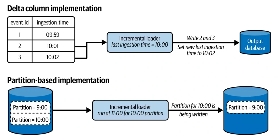
- Delta column: to identify rows added since the last run. the delta column implementation needs to remember the last ingestion time value to incrementally process new rows.
- Time-partitioned datasets: the ingestion job uses time-based partitions to detect the whole new bunch of records to ingest.
Consequences
- Hard deletes
  - Using the pattern can be tricky for mutable data. Specifically for updated and deleted process. Where if deletes a row, the information physically disappears from the input dataset. To overcome this issue we can rely on soft deletes, where the producer, instead of physically removing the data, simply marks it as removed. Put differently, it uses the UPDATE operation instead of DELETE.
- Backfilling
  - To prevent changing between increment process to full load process due to backfilling, we could limiting the ingestion window.
  - This operation brings two things:
    - Better control over the data volume
    - Simultaneous ingestion.
Example
- Script, applies to the incremental load and deploy it to our runtime service
- Apache Airflow and Apache Spark: Using File Sensor and once the partition is ready, the pipeline triggers the data ingestion job.

Change Data Capture

This pattern has better for a lower ingestion latency or built-in support for the physical deletes.

The latency requirement makes it impossible to use the Incremental Loader. The pattern has some job scheduling and query execution overheads that could make the expected latency difficult to reach. A better candidate is the Change Data Capture (CDC) pattern. Due to its internal ingestion mechanism, it guarantees lower latency. The pattern consists of continuously ingesting all modified rows directly from the internal database commit log. It allows lower-level and faster access to the records, compared to any high-level query or processing task.

A commit log is an append-only structure. It records any operations on the existing rows at the end of the logfile. The CDC consumer streams those changes and sends them to the streaming broker or any other configured output. From that point on, consumers can do whatever they want with the data, such as storing the whole history of changes or keeping the most recent value for each row.

Besides guaranteeing lower latency, CDC intercepts all types of data operations, including hard deletes. So there is no need to ask data producers to use soft deletes for data removal.

Consequences
- Complexity
  - The CDC pattern may need some help from the operations team, for example, to enable the commit log on the servers.
- Data scope
- Payload
  - CDC will bring additional metadata with the records, such as the operation type (update, insert, delete), modification time, or column type.
- Data semantics
  - Data in motion has different processing semantics for many operations that appear to be trivial in the data-at-rest world.
  - Example: when joining 2 data with or without streaming source, there will be some issues mainly in delay process.
Example
- Create our own commit log reader
- Debezium + Kafka Connect

Replication

The main goal of which is to copy data as is from one location to another. Replication is about moving data between the same type of storage and ideally preserving all its metadata attributes, such as primary keys in a database or event positions in a streaming broker.

Passthrough Replicator

Similar with pass-through job expecially in separate environments e.g.: development, staging, and production.

Implementation level
- The compute level implementation relies on the EL job, which is a process with only two phases, read and write. Ideally, the EL job will copy files or rows from the input as is (i.e., without any data transformation).
- The infrastructure level part is based on a replication policy document where we configure the input and output location and let our data storage provider replicate the records on our behalf.
Consequences
- Keep it simple
  - The main goal is get the data as is. To reduce the interference risk in the replicated dataset, we should rely on the simplest replication job possible, which is ideally the data copy command available in the database.
  - Use the simpler raw text API that will take and copy lines as they are, without any prior interpretation.
- Security and isolation
  - implement the replication with the push approach instead of pull to manage risk such as stability issue.
  - Push apporach means that the environment owning the dataset will copy it to the others and thus control the process with its frequency and throughput.
  - PII data
    - Use the Transformation Replicator pattern that adds an extra transformation step to get rid of any unexpected attributes.
  - Latency
    - The infrastructure-based implementation often has some extra latency, and we should always check the service level agreement (SLA).
  - Metadata
Example
- Using Distributed data processing framework
- A data copy utility script running on our storage layer
- Apache Spark: synchronize semi-structured JSON files
- Apache Kafka: requires an extra ordering guarantee within the partitions.
- the infrastructure-based: MirrorMaker utility for topic replication, replication mechanism tools (e.g. Terraform).

Transformation Replicator

Performing tests against real data to avoid surprises during production. We can’t use a synthetic data generator because our data provider often has data quality issues and it’s impossible to simulate them with any tool. We have to replicate the data from production to the staging environment. Unfortunately, the replicated dataset contains PII data that is not accessible outside the production environment.

We should implement the Transformation Replicator pattern, which, in addition to the classical read and write parts from the Passthrough Replicator pattern, has a transformation layer in between.

The transformation consists of either replacing the attributes that shouldn’t be replicated (for example, with the Anonymizer pattern) or simply removing them if they are not required for processing.

Consequences
- Transformation risk for text file formats
  - Example: the datetime format is different from the standard used by our data processing framework. Instead of defining the timestamp columns as is, we can simply configure them as strings and not worry about any silent transformations.
- Desynchronization
  - Data is continuously evolving, and nothing guarantees that the privacy fields we have today will still be valid in the future. Maybe new ones will appear or attributes that are not currently considered PII will be reclassified as PII.
  - To avoid these kinds of issues, if possible, we should rely on a data governance tool, such as a data catalog or a data contract in which the sensitive fields are tagged.
Example
- Databricks and BigQuery (or SQL): data reduction approach that eliminates unnecessary fields
- PySpark: drop function
- AWS Redshift: GRANT SELECT
- Apache Spark: mapping function

Data Compaction

Even a perfect dataset can become a bottleneck, especially when it grows over time because of new data. As a result, at some point, metadata-related operations like listing files can take even longer than data processing transformations.

Compactor

The easiest way to address this issue of a growing dataset is to reduce the storage footprint of the underlying files.

E.g. real-time data ingestion pipeline synchronizes events from a streaming broker to an object store. The main goal is to make the data available for batch jobs within at most 10 minutes. Since it’s a simple passthrough job, the pipeline is running without any apparent issues. However, after three months, all the batch jobs are suffering from the metadata overhead problem due to too many small files composing the dataset. This will spend 70% of execution time on listing files to process and only the remaining 30% on processing the data. This has a serious latency and cost impact as our use pay-as-you-go services.

Having small files is a well-known problem in the data engineering space. Storing many small files involves longer listing operations and heavier I/O for opening and closing files. A natural solution to this issue is to store fewer files.

Compactor pattern addresses the problem by combining multiple smaller files into bigger ones, thus reducing the overall I/O overhead on reading. Open table file formats have their dedicated compaction command that often runs a transactional distributed data processing job under the hood to merge smaller files into bigger ones as a part of the new commit.

Examples
- Apache Iceberg: rewrite data file action
- Delta Lake: OPTIMIZE and VACUUM command
- Apache Hudi: merge-on-read (MoR) table
- Apache Kafka: append-only key-based logs system
Consequences
- Cost versus performance trade-offs
  - The compaction job is just a regular data processing job that can be compute intensive on big tables.
  - If we consider only this aspect, we should execute it rarely, such as once a day, ideally outside working hours, and outside the pipeline generating the dataset.
  - We’ll then need to choose our strategy and accept that it may not be perfect from both the cost and performance perspectives. There is no one-size-fits-all solution.
- Consistency
  - Compaction simply rewrites already existing data. Consequently, consumers may have difficulties distinguishing the data to use from the data being compacted.
  - Compaction is much simpler and safer to implement in modern, open table file formats with ACID properties (such as Delta Lake and Apache Iceberg) than in raw file formats (such as JSON and CSV).
- Cleaning
  - The compaction job may preserve source files. We’ll have to complete it with a cleaning job to reclaim the space taken up by the already compacted files.

Data Readiness

This part will answer problematic question we’ll certainly ask ourself is, “When should We start the ingestion process?”

Readiness Marker

The Readiness Marker is a pattern that helps trigger the ingestion process at the most appropriate moment. Its goal is to guarantee the ingestion of the complete dataset.

E.g. In data lineage, there will be some process that need a dynamic time to execute. It will arise an issue such as: complain about incomplete datasets, and they’ve asked us to implement a mechanism that will notify them directly or indirectly—when they can start consuming our data.

The issue is particularly visible in the logically dependent but physically isolated pipelines maintained by different teams. Because of these isolated workloads, it’s not possible for our job to directly trigger downstream pipelines. Instead, we can mark our dataset as ready for processing with the Readiness Marker pattern.

The first implementation uses an event to signal the dataset’s completeness.

Example
- Apache Spark: flag file
- Delta Lake: new commit log
- the data orchestration layer: as a separate task executed after successful data processing.

A different implementation applies to partitioned data sources.

If we’re generating data for time-based tables or locations, the Readiness Marker can be conventional. E.g. update hourly base partition, and get the latest update after each hour.

Consequences
- Lack of enforcement
  - There is no easy way to enforce conventional readiness based on the flag file or the next partition detection. It’s very important to communicate with our consumers and agree upon the conditions that may trigger processing on their side. Clearly explain the risks of not respecting the readiness conventions.
- Reliability for late data
  - If the partitions are based on the event time, the partitionbased implementation will suffer from late data issues.
  - That’s why we should either consider partitions as immutable parts that will never change once closed or clearly define and share the mutability conditions with our consumers.

Event Driven

The Readiness Marker pattern from the previous section relies on pull semantics, in which the consumer is responsible for checking whether there is new data to process.

It’s hard to predict the incoming frequency of data. Consequently, we must shift our mindset from static ingestion to event-driven ingestion.

External Trigger

The event-driven nature of a dataset favors push semantics, in which the producer is in charge of notifying consumers about data availability.

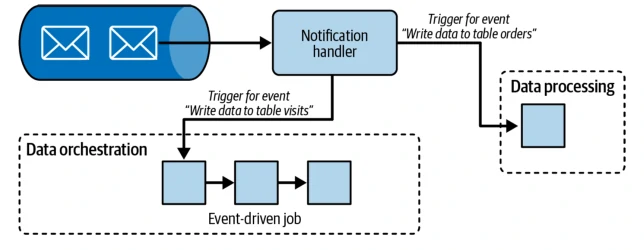
With the goal of reducing costs, we want to change the scheduling mechanism and run the pipeline only when there is something new to process. The prosedure sends a notification event to a central message bus with specific topic and it will be distribute to each consumer for each topic.

Three main actions:
- Subscribing to a notification channel.
- Reacting to the notifications. The role of this stepis to analyze the event and decide whether:
  - It should result in triggering a pipeline in the data orchestration layer
  - Starting a job in the data processing layer.
- Triggering the ingestion pipeline in the data orchestration or data processing layer.
Consequences
- Push versus pull
  - The External Trigger component can implement pull or push semantics. The difference is the key in understanding the pattern’s impact on our system.
  - The pull-based trigger continuously checks whether there are new events to process, while the push-based trigger does nothing as long as the event producer doesn’t notify it about something new to process.
  - The pull-based trigger is a long-running job, so it’s a process that stays up and checks at short, regular intervals whether there is new data to process. It’s not the most optimized since the job may spend most of its time pulling zero messages from the notification source.
  - The push-based trigger, where the data source informs the endpoint(s) about new messages present in the bus. Each notification message starts a new consumer instance which finishes after reacting to the event.
- Execution context
  - There is a risk that the external trigger may become just a ping mechanism that calls a data orchestrator endpoint.
  - It’s important to enrich the triggering call with any appropriate metadata information, including the version of the trigger job, the notification envelope, the processing time, and the event time. They will be useful in day-to-day monitoring, when we will need to investigate the reasons for any eventual failures.
- Error management
  - The events are the key elements here, and without them, we won’t be able to trigger any work. We should design the trigger for failure with the goal in mind to keep the events whatever happens.
Example
- Could-based event driven: AWS, Azure, and GCP provide serverless function services.
- Data orchestrators expose an API that we can use to start a pipeline. (AWS Lambda function with Apache Airflow).

drawing

Error Management Design Patterns

While processing the data, we’ll face two kinds of errors.

Transient errors: that are often temporary and will eventually recover automatically in the future. (a short database unavailability mitigated with automatic connection retries).
Nontransient errors: that are not temporary and will never recover by themselves. (unprocessable records or poison pill messages). They are fatal issues that stop the application and require our manual intervention.
Unprocessable Records

Dead-Letter

An easy solution is to ignore the bad records and continue processing the correct ones. It’s easy to do if we can simply skip the invalid events and thus lose them forever. Or we can opt for another approach and save the bad records elsewhere for further investigation.

The solution should keep the pipeline running even for the occasional failed records and give us an opportunity to investigate the errors later.

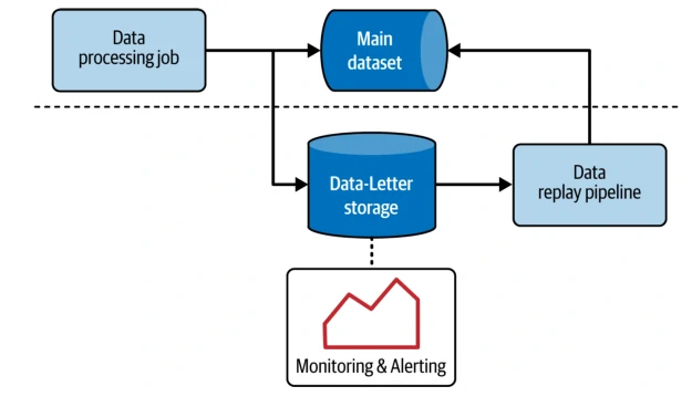
Workflow
- Identifying places in the code where our job can fail.
- Add some error handling logic / safety controls over the likely fail spots that have been identified. (try-catch block or if-else condition).
- Add the failed message as the metadata to help us better understand the failure at the post-analysis stage.
- Configure a the dead-letter storage for the erroneous events. Consider the following for destination of the erroneous events:
  - Resiliency, so that we don’t need to think about a dead-letter strategy for our dead-letter storage.
  - Monitoring ease, to better understand whether the errors are only occasional issues or whether the whole system is going down.
  - Writing performance, since writing the unprocessed records to an extra place will incur some cost in the overall job execution time.
  - Good candidates for the dead-letter stores are object stores in the cloud or streaming brokers since they’re highly available, fast, and easy to be the monitoring layer.
- Add the replay pipeline that ingests the failed records into the main data flow.

The difference between implementing Dead-Letter at stream processing and batch workloads comes from the data perception.

Streaming operates on one record at a time and thus can write an individual record to dead-letter storage.
Batch works on a bunch of data, and very often, it will write a subset of the erroneous records at once to dead-letter storage.
Consequences
- Snowball backfilling effect
  - The good thing about the fail-fast approach is its simplicity for the whole system. On the other hand, if our job doesn’t follow the fail-fast strategy, consumers will continue processing data that might be partial.
  - If we decide to run the replay pipeline, the ingested records can belong to the partitions already processed by our downstream consumers. That would require a back-filling action on their part and start a snowball backfilling effect, where their downstream consumers must reprocess the data as well. Mitigating this issue is not easy because each solution comes with its own trade-offs.
- Dead-lettered records identification
  - It better to distinguish dead-lettered records from the rows added in the normal ingestion pipeline.
  - It can be useful to implement a filtering condition skipping replayed records in the downstream consumers or to simply track the origin of each row.
  - We can add a boolean column or an attribute called was_dead_lettered to indicate each record produced by the Dead-Letter replay job.
- Ordering and consistency
  - The pattern can break data consistency. E.g. break session due to dead-letter for the range of time.
  - This is also true for the ordered data delivery requirement. In that case, any replayed failed delivery will break the ordering consistency.
- Error-safe functions
  - When we use error-safe functions, instead of capturing the exception, we’ll need to compare the output value with the input. If the input is present but the function returns a NULL value, it might represent a processing error and thus an unprocessable record.
  - We need to understand their error-safety semantics, which may differ from one function to another.
- Error or failure?
  - This pattern will hide a fatal failure that should stop the pipeline.
  - We should complete the code implementation with an appropriate alerting layer that, in case of too many dropped events, could stop the job to avoid propagating potentially wrong data to our system.
Examples
- Apache Flink: side outputs
- Apache Kafka: try-catch block / if-else condition
- Batch: try-catch block / if-else condition
- Apache Spark SQL and Delta Lake: error-safe CONCAT data transformation

Duplicated Records

Duplication records could be happen in distributed systems, backfilling process in error management, or system behaviour.

Exactly-once processing works only if we don’t encounter runtime errors. Otherwise, the restarted job execution may reprocess already processed records, despite the deduplication logic. This is often an accepted trade-off between automated transient errror managent and deduplication.

Exactly-once processing doesn’t guarantee exactly-once delivery or perfect deduplication

Windowed Deduplicator

The key for data deduplication is to consider the data to be limited.

The streaming jobs, the limits will be time-based windows.

The batch jobs will reduce the scope to the currently processed dataset.

Workflow
- Identifying the deduplication attributes that guarantee the uniqueness of each record.
- Define the deduplication scope, to limiting compute power and slow process.
- Execute the data
Consequences
- Space versus time trade-off
  - This is a main consequnces of streaming pipelines, a short window will probably miss some duplicates, but on the other hand, it will have a small impact on resources.
- Idempotent producer
  - Correctly deduplicating the data doesn’t guarantee exactly-once delivery for processed records. Very often, it will not be possible because of transient errors and their automatic solutions, such as retries.
Example
- Apache Spark: dropDuplicates function (for both batch and streaming jobs)
- Batch jobs - SQL
  - DISTINCT expression
  - WINDOW function alongside the condition on the row_number()
- Streaming jobs
  - Using the state store to verify whether a record has already been seen or not.
  - types of state stores. They’re all trade-offs between performance and data consistency:
    - Local: the state data lives only in memory.
    - Local with fault-tolerance: the state still primarily lives in memory and the job persists it to a remote storage for fault tolerance reasons.
    - Remote: the state is only present in a remote data store.

Late Data

Late Data Detector

The first step when dealing with data arrival issues is their detection with the Late Data Detector pattern. It can help in many situations, such as completing already processed partitions or controlling the state in stateful jobs, as we saw before for deduplication in stream processing.

Workflow
- The pattern requires defining one time-based attribute to track late data. The attribute should describe when a given event happened. Otherwise, it might be impossible to classify the incoming records as being late or on time.
- Define a latency aggregation strategy that will apply individually to each partition in our input data store. To avoid a situation in which our processing layer doesn’t move on, the latency aggregation strategy must be monotonically increasing. The most common aggregation strategy uses the MAX function, taking the greatest event time for each partition.
- Decide on an additional aggregation strategy that will calculate a single event time for all partitions to represent overall progress.
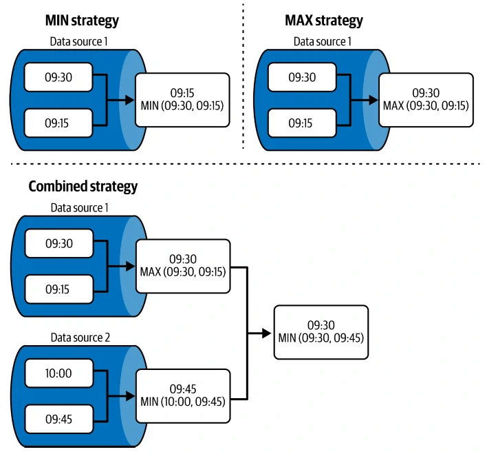
  - For this global event time, we can opt to use the following:
    - The MIN function if our job needs to follow the slowest upstream dependency.
    - The MAX function that follows the fastest upstream dependency.
    - The MIN and MAX combined at different levels.
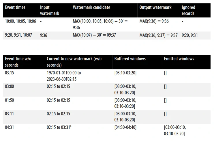
- Add an allowed lateness attribute to allow some extra unexpected latency. The Late Data Detector pattern subtracts the allowed lateness value from the workflow’s tracked event time as MAX(event time) - allowed lateness. The result of this calculation is called the watermark, and it defines the minimum event time to consider an event as on time.
Example for watermark could be shown below.
Consequences
- Prebuild Late data capture tool
- MIN strategy, stuck-in-the-past situations, and stateful jobs
  - The partition-based event time tracker doesn’t use the MIN function in order to avoid a stuck-in-the-past situation.
  - If we used the MIN strategy to track partition event times, it would imply the following consequences:
    - Open-close-open infinite loop
    - Stuck in the past: If our pipeline is getting late data over and over again, the watermark may never make any progress. Consequently, our eventual event time–based state will grow because we will not be able to determine the buffered items as completed with regard to the watermark.
- Max strategy and event skew
  - In highly skewed environments, it can be too aggressive and consequently drop many records. Unfortunately, there is no silver bullet for this issue. The best mitigation strategy should rely on appropriate late events monitoring and the possibility of reintegrating late records whenever there is a high event skew.
Example
- Apache Spark Structured Streaming: withWatermark function. A built-in capability to detect and ignore late events, but it doesn’t expose an API to capture them easily.
- Apache Flink: provides more flexibility for both capturing and detecting late events.

Static Late Data Integrator (Circuit Breaker / CQRS)

By default, we can ignore late data. However, late data may also be valuable, and if it represents a significant percentage of our dataset, losing it won’t be an option.

A fixed delay for late data ingestion is a perfect scenario where we can leverage the Static Late Data Integrator pattern.

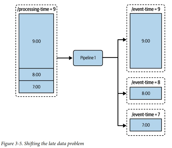
The easiest solution to the problem is using processing time–based partitions. However, if we do care about the event time somewhere in our system, using the processing time solution simply moves the problem somewhere else.

E.g. processing time partition for nine o’clock has the following distribution: 80% of the data for nine o’clock, 10% for eight o’clock, and 10% for seven o’clock. One of the downstream consumers uses event time–based partitions. Hence, even though our pipeline doesn’t need to deal with late data, it generates late data that will need to be handled by other processes in the system.

Start the implementation by defining a so-called static lookback window (i.e., how far to look back in the past for late data in a given job execution) with fix window duration.

drawing

After defining the lookback window, we need to place the late data integration process in our pipeline.

drawing

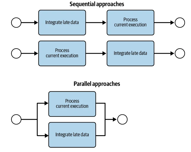
Some strategic that we can apply to handle this the late data integration process:

the sequential strategy: this is for stateful pipelines where the results generated by one execution depend on the results generated by the previous executions.
For stateless pipelines, we can use and switch between all three strategies. But if we want to deliver current data first, we should opt for either the second or the third approach, in which late data is handled at the same time or after the current execution time.

detect data that belongs to a period that has already been processed, identify the affected keys or partitions, and apply targeted corrections rather than rebuilding the entire dataset.

Difference from Watermark
- Watermark
  - Accept data until
  - T + 10 minutes
  - After that
  - Drop it
- Static Late Data Integrator
  - Accept forever
  - Correct historical data
ELI5
- Imagine a teacher collects homework every day.
  - At 5 PM, she grades all homework that has arrived.
  - Some students submit late the next morning.
  - Instead of re-grading the entire class, she has a separate notebook.
- Whenever late homework arrives:
  - Find the student’s previous score.
  - Replace it with the corrected score.
  - Update the final report.
- The homework already graded is the static dataset.
- The late homework is the late data.
- The notebook used to merge them is the Static Late Data Integrator.
- The word Static refers to the fact that the primary dataset has already been finalized.
- Rather than recomputing all data that already calculated, we integrate only this new record into the static table.
Implementation
- MERGE INTO
- UPSERT
- DELETE + INSERT

Use Case

Original data

OrderID Revenue

1 100

2 200

3 300
Daily total: 450

OrderID	Revenue
1	100
2	200
3	300

Two days later

  Late Order

  OrderID=4
  Revenue=300
  Date=Yesterday

Static Late Data Integrator

Find yesterday
Current Total = 450
450 + 300 =750
Update yesterday only

No need to recompute every day.

Static Late Data Intergrator (IoT)

Load 10:00-10:05 window
Insert event
Recalculate average
Overwrite window

Static Late Data Intergrator (IoT)

Reload July 1
Recalculate
Publish corrected balance

Architecture

           Streaming Events
                    │
                    ▼
           Real-time Aggregation
                    │
                    ▼
          Final Daily Sales Table
            (Static Dataset)
                    │
        --------------------------
        │                        │
  Late Event Stream         Historical Table
        │                        │
        └──────────┬─────────────┘
                   ▼
        Static Late Data Integrator
                   │
                   ▼
         Corrected Historical Table

The historical table is mostly immutable. Only affected records are updated.

Consequences
- Snowball backfilling effect
  - If we are a data provider and our data consumers care about consistency, they’ll inevitably need to replay all partitions with the late data, just as we have done. If they have consumers too, those consumers will also need to run backfilling for these partitions…and in the end, the whole operation may become very compute intensive.
- Overlapping executions and backfilling
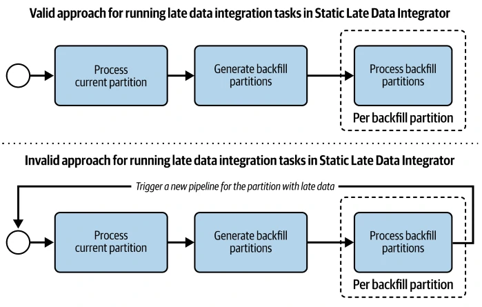
  - we shouldn’t backfill our jobs as we would backfill jobs without the static lookback window.
- Pipeline trigger
  - With the Static Late Data Integrator, our backfilling jobs must be part of the main pipeline. We can’t start separated pipelines as part of the lookback window–based backfilling because it’ll lead to the same problem as overlapping executions and backfilling.
- Waste of resources
  - Fixed periods from the lookback window may not contain late data every time. We can add a control task to run the integration task only when there is late data.
- Time requirement
  - If our dataset is not partitioned by time or doesn’t have any time concept, we cannot really detect and thus integrate late data. Time partitions from the Static Late Data Integrator pattern are time boundaries that each incoming record is comparing against.
- Downstream consistency
  - Reports may already have consumed old values. Need:
    - versioning
    - CDC
    - refresh strategy
Example
- Apache Airflow: Dynamic Task Mapping. The feature lets us create tasks dynamically from a data provider function. A perfect fit for generating late data integration tasks for the static lookback window duration.

Dynamic Late Data Integrator

Having a static tolerance period is not always possible, and sometimes we may need a more dynamic approach that will just load the partitions impacted by the late data.

Using Dynamic Late Data Integrator patter to handle variability and integrate only the partitions with late data. The implementation leverages a lookback window that is dynamic, which means that all the backfilled partitions really contain late data. To make this happen, the dynamic approach requires an additional data structure to store the last execution time, and eventually, the last update time for each partition.

drawing

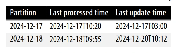
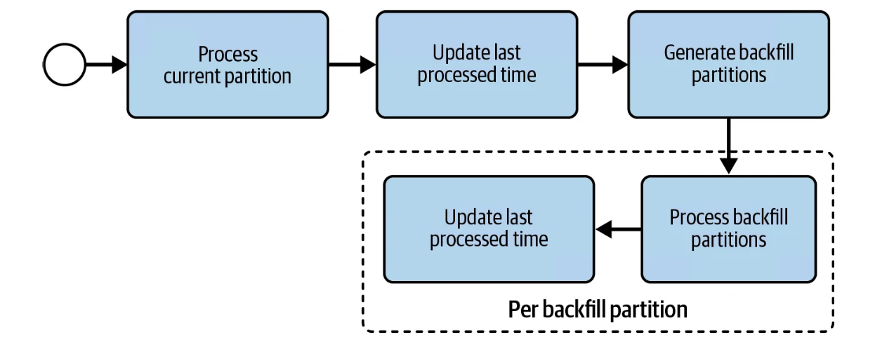
Consequences
- Concurrency
  - If our pipeline supports concurrent executions, dynamic late data integration may generate duplicated late data integration runs.
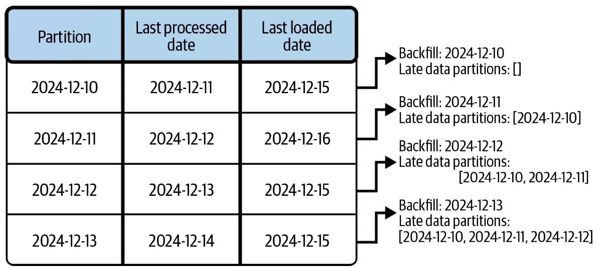
  - Shows what could happen in a pipeline running four different jobs in parallel, with late data in each processed partition.
  - We need to add an extra column to the state table that will keep the partition status either as already processed or as being processed. -
  - Consequently, the query retrieving the partitions to backfill should add this column as an extra filtering condition to ignore the partitions already planned for late data integration.
  - Each pipeline needs to start with the task that updates the is_processed column of the currently processed partition. That way, we can avoid having the next execution generate the current partition as the one to backfill. Also, this task should run only if the execution of the previous run succeeded.
  - The task that generates the partitions to backfill should now also update all retrieved partitions as having been processed. It should run only if its previous execution succeeded. This dependency on the past runs helps avoid race conditions and triggering the same partitions in two different runs.
  - The task updating the last processed time should additionally set the Is processed flag to false. That way, if the partition gets new late data, it can still be replayed.
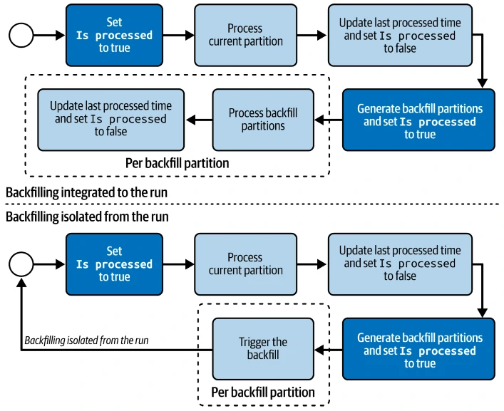
  - If the task that generates partitions to backfill fails, its future executions will not run due to the dependency on the previous run. Consequently, the pipeline will get stuck in a long in-progress state requiring our manual intervention to unblock it.
- Stateful pipelines and very late data
  - with the last successful run having taken place on 2024-10-20. There hasn’t been any late data so far, but the next day’s execution spots late data ingested for the partition of 2024-09-21.Since our job is stateful, we will need to regenerate all executions from 2024-09-21 to 2024-10-20 to guarantee the correctness of our dataset.
- Scheduling complexity
  - Depending on our storage layer, getting the last modification time for each partition might not be easy. This step can involve dealing with the internal details of a storage technology or even implementing the update tracking table on our own.
Example
- Apache Airflow: Dynamic Task Mapping. depends_on_past attribute.
- Delta Lake: DeltaLog class

Filter

Filter Interceptor

TBN

Fault Tolerance

A form of protection that ensures recoverability for continuous data processing workflows, such as streaming ones. The challenge with these workflows is to know when to start after stopping the job.

Checkpointer

The fatal error is particularly critical in stream processing. These applications are working on continuously arriving events that are often stored in an appendonly log.

To avoid reprocessing past data, our job must keep track of the most recent position in the consumed data source, as well as the computed state. The Checkpointer pattern implements this tracking mechanism.

Checkpointing consists of recording the data processing process in a more persistens storage than the job’s environment, which may change when we restart it.

Approaches
- Data processing framework based
  - Rely on a data processing framework, the progress information may be recorded in the environment managed by the framework itself.
- Data store based
  - Using the data store SDK, we may be interacting with the data store layer for the checkpoint information.
Implementations
- Configuration driven: where we only configure the checkpointing frequency and delegate the execution to our library.
- Intentional checkpointing action from the code. Here, after reading and processing the records, wou’ll be responsible for confirming this operation to avoid getting the same data in the next execution.
Example
- Apache Spark Structured Streaming and Apache Flink: store the progress metadata. The checkpointLocation attribute.
- Apache Kafka SDK: __consumer_offsets
- Amazon Kinesis Client Library (KCL): checkpoint Amazon DynamoDB table.
Consequences
- Delivery guarantee versus latency trade-off
  - Position tracking is not an expensive operation in terms of latency. It only accumulates some numbers for each input partition in memory and persists them once in a while to a persistent storage.
  - Tracking the state may have a more significant latency impact as the state will probably be many times bigger than those numeric positions.
  - we’ll need to balance the latency requirements and the processing guarantee. The more frequent the checkpoints are, the slower the job will be due to checkpoint creation overhead.
- Exactly-once feeling
  - There could be multiple tasks working in parallel and in an asynchronous manner. If one of them fails in the middle of the work before triggering the checkpoint, the restart will involve retries and reprocessing of the already successful records.

Idempotency Design Patterns

Idempotency is the process that return no matter how many times we invoke the function, we always get the same result. It’s a way to ensure that no matter how many times we run a data processing job, we’ll always get consistent output without duplicates or with clearly identifiable duplicates.

Avoiding duplicates will not always be possible. If we generate the data to a messaging system that doesn’t support transactional producers, retries can still generate duplicated entries. But this issue could be handle at consumers side that will be able to indetify those records as such.

Overwriting

The first idempotency family covers the data removal scenario. Removing existing data before writing new data is the easiest approach. However, running it on big datasets can be compute intensive. For that reason, to handle the removal, we can use data- or metadata-based solutions.

Fast Metadata Cleaner

Metadata operations are often the fastest since they don’t need to interact with the data files. We often say that the metadata part operates on the logical level instead of the physical one.

To achieve idempotency, the Fast Metadata Cleaner pattern relies on dataset partitioning and data orchestration. We need to define the partitioning carefully since it directly impacts the idempotency granularity.

Granularity defines at the same time the units on top of which we can apply the metadata operations to clean the table. It has an important consequence for backfilling.

This pattern could be used at incremental and partitioned datasets or full dataset.

The adaptation consists of adding these extra steps
- Analyze the execution date and decide whether the pipeline should start a new idempotency granularity or continue with the previous one.
- Create the idempotency environment.
- Update the single abstraction exposing the idempotency context tables.

drawing

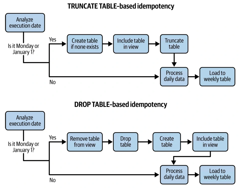
Consequences
- Granularity and backfilling boundary
  - The pattern defines an idempotency granularity that is also a backfilling granularity.
  - If we replay the pipeline, we have to do it from the task that creates a partitioned table. Otherwise, we’ll end up with an inconsistent dataset.
  - if we partition the data on a weekly basis and we need to backfill for only one day, we have no choice but to rerun the whole week. This doesn’t mean we’ll have to reprocess full pipelines for other days, though. If only one day generated an invalid dataset, it’s enough to replay only the data loading step for the remaining days.
- Metadata limits
  - Also be aware of the limits of our data store. The pattern relies on creating dedicated partitions or tables, but unfortunately, it often won’t be possible to create them indefinitely.
  - To overcome these limitation issues, we can add a freezing step to transform the mutable idempotent tables into immutable ones, thus reducing the partition scope. For example, weekly tables could turn into monthly or yearly tables if there are no possible changes after a freezing period.
- Data exposition layer
  - The final point is about access. The dataset is not living in a single place anymore, and our end users may not want to know the internal details of the design and may instead prefer to access the data from a single point of entry.
  - Use a solution similar to a database view, such as a logical structure grouping multiple tables and exposing them as a single unit.
- Schema evolution
  - Another challenge is schema evolution. If our idempotency tables get a new optional field, we’ll need a separate pipeline to update the schema of already existing tables.
Example
- Scripts: Remove / secure the rows DELETE operation, inserts processed rows INSERT operation. Or better process using TRUNCATE or DROP operation.
- Apache Airflow + PostgreSQL table: BranchPythonOperator + PostgresViewManagerOperator operator.

Data Overwrite

If using a metadata operation is not an option, we need to apply a data operation. When the metadata layer is unavailable or using it involves a lot of effort, we can rely on the data layer and the Data Overwrite pattern.

Running the overwriting command doesn’t guarantee our data will disappear. If we use a data store–supporting time travel feature, thus making it possible to restore the dataset to one of its past versions, the data blocks will still be there after we execute the overwrite. They will only be deleted after the configured retention period or after running the vacuum operation to reclaim unused space if the command is supported.

Solution
- A data processing framework
  - We may simply need to set an option while configuring our data writer. Once we’ve configured our data writer, the data processing framework will do the rest (i.e., cleaning the existing files before writing).
- work directly with SQL
  - use a combination of DELETE FROM and INSERT INTO operations.
  - A more concise alternative to DELETE and INSERT leverages the INSERT OVERWRITE command. This alternative overwrites the whole table with the records from the INSERT part of the statement. INSERT OVERWRITE doesn’t support selecting rows to overwrite, whereas the combination of DELETE and INSERT operations does.
  - Use the data loading commands available in our data store. such as LOAD DATA OVERWRITE in BigQuery, support data overwriting natively. The others should be preceded with a TRUNCATE TABLE command.
Example
- Apache Spark: save mode, .write.mode('overwrite').
- Apache Flink: the write mode properties
- Delta Lake: replaceWhere option
- Databricks and Snowflake: INSERT OVERWRITE command.
- BigQuery: writeDisposition in the jobs feature, --replace=true flag.
- SQL:
  - DELETE FROM and INSERT INTO operations.
  - INSERT OVERWRITE command.
  - LOAD DATA OVERWRITE in BigQuery.
  - TRUNCATE TABLE command.
Consequences
- Data overhead
  - Since there is a data operation involved, the pattern can perform poorly if the overwritten dataset is big and not partitioned. We can try to mitigate this overhead by applying some storage optimizations, like partitioning. They should reduce the volume of data to overwrite and hence make the replacement action faster.
- Vacuum need
  - A DELETE operation might not remove the data immediately from the disk. This happens with table file formats and relational databases, where deleted data blocks, albeit not accessible by users with SELECT queries, still exist on disk.
  - To reclaim the space occupied by these dead rows, we will need to run a vacuum process that will remove them for real.

Updates

This is the case with updated incremental datasets, in which each new version generated by our data provider contains only a subset of modified or updated data. If we try to rewrite the whole dataset, we’ll have to do some preparation work to keep only the most recent version of each entity.

Merger

In a nutshell, If we don’t have the complete dataset available —for example, if we’re working with the incremental changes streamed from a database in our problem statement— we need to consider combining changes with an existing dataset. that’s what the Merger pattern does.

The Merger pattern, requires us to interact with the data to combine new and existing rows.

Workflow
- Define the attributes we’re going to use to combine the new dataset with the old one. We can use a single property —such as the user ID— or combination of several properties, if it guarantees uniqueness across the dataset.
- Find a way to combine datasets in our processing layer. The common one is the MERGE (aka UPSERT) command.
- Define the behavior for each of the possible scenarios, which are as follows:
  - Insert: The entry from the new dataset doesn’t exist in our current dataset. Therefore, it’s a new record we have to add.
  - Update: Both datasets store a given record, but it’s very likely that the new dataset will provide an updated version of the record.
  - Delete: This is the trickiest case because the Merger pattern doesn’t support deletes. If a record is missing from the dataset we want to merge, nothing will happen. For that reason, deletes are only possible if they’re expressed as soft deletes (i.e., updates with an attribute marking a given record as removed). That way, we can detect the change and apply a hard or soft delete to our data.
- the MERGE statement covering all three scenarios.

Code

MERGE INTO dedp.devices_output AS target
USING dedp.devices_input AS input
ON target.type = input.type AND target.version = input.version
WHEN MATCHED AND input.is_deleted = true THEN
DELETE
WHEN MATCHED AND input.is_deleted = false THEN
UPDATE SET full_name = input.full_name
WHEN NOT MATCHED AND input.is_deleted = false THEN
INSERT (full_name, version, type) VALUES (input.full_name, input.version, input.type)

Consequences
- Uniqueness
  - This is the first and most important requirement. The data must define some immutable attributes we can use to safely identify each record. Otherwise, the merge logic will simply not work because instead of updating a row in case of backfilling, it might insert a new one, leading to inconsistent duplicates.
I/O
- Merger is a data-based pattern. It works directly at the data blocks level, which makes it more compute intensive.
Incremental datasets with backfilling
- We need to be aware of a shortcoming of the Merger pattern in the context of backfilling. In case of incremental dataset, the backfill will start from the most recent version, and leads to some of them are missing in the parts of the table at the time backfilling will occur. To mitigate this issue, we may need to implement a restore mechanism outside the pipeline that will roll back the table to the first replayed execution. It’s relatively easy to do if the database natively supports this versioning capability.
Example
- Apache Airflow + SQL query: MERGE + UPDATE + WHEN NOT MATCHED THEN + WHEN MATCHED THEN +INSERT operation.
- Script: UPSERT operation.

Stateful Merger

The Merger pattern lacks some consistency for datasets during the backfillings. If consistency is important, we can use stateful merger pattern.

Whenever we need to restore a dataset, the Merger pattern won’t be enough because it focuses only on the merge action. But there is an alternative called a Stateful Merger pattern that provides data restoration capability via an extra state table.

This extra state table involves some changes in the pipeline. The workflow now has an additional step in the beginning to restore the merged table if needed and another at the end to update the state table.

Workflow
- The merge operation completes, it creates a new version of the merged table.
- The completion also triggers another task that retrieves the created table version and associates it with the pipeline’s execution time.
- The restore process will happen only when the pipeline runs in the backfilling mode. Otherwise, it will do nothing.
- To implement this backfilling detection logic, our data orchestrator should provide a context for the execution, and from this context, we can learn about the execution mode (backfilling or normal run), we can simply analyze this context metadata.
- If that’s not the case, we need to implement some logic leveraging the state table. The high-level logic consists of the following:
  - Getting the version of the table created by the previous pipeline’s run. If this version is missing, it means we’ll run the pipeline for the first time or backfill the first pipeline’s execution.
  - Comparing the current dataset version with the dataset version created by the previous pipeline’s execution.
  - If the two versions are the same, there is nothing to restore as the pipeline is running in the normal mode.
  - If the two versions are different, it means the pipeline has entered into the backfilling scenario.
Consequences
- Versioned data stores
  - The presented implementation of the Stateful Merger pattern requires our data store to be versioned. That’s the only way we can track the state and restore the table to a prior version. If we don’t work on a database with versioning capabilities, such as table file formats, we should slightly adapt the implementation to our use case.
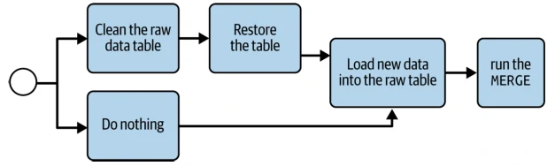
  - Instead of versioning the table, the pipeline loads all raw data into a dedicated raw data table with a column storing the execution time. The backfilling detection logic verifies whether the raw data table has some records for the execution times in the future.
- Vacuum operations
  - After the configured retention duration, they remove files that are not used anymore by the dataset. Consequently, some of the prior versions will become unavailable at that moment.
- Metadata operations
  - Compaction doesn’t overwrite the data but only combines smaller files into bigger ones. But despite this no-data action, it also creates a new version of the table. As a result, if we always use the previous version from the state table in the restore action, we will miss the operations made between two merge runs.
Example
- Apache Airflow: the job’s execution time + delta table version created retrieves the table version
- Delta Lake
- Apache Spark: spark.sql operation

Database

Rely on the databases to guarantee idempotency.

Keyed Idempotency

This pattern uses key-based data stores and an idempotent key generation strategy. This mix results in writing data exactly once, no matter how many times we try to save a record.

In the context of a key-based database, idempotency applies to the key generation logic on the data processing side. When it comes to the actual implementation, we should start by finding immutable properties for the key generation. Our input dataset may already have unique attributes for our use case.

However, the key may not always be available. Instead, we could use the combination of e.g. the user ID and the first visit time to generate an idempotent key. Although this is a valid solution, if our job stopped because of an unexpected runtime error, and after the restart, the session ID changed because of late data written to the input data store.

In the context of idempotent key generation for a user session, the event time attribute is mutable (i.e., the value may change between runs). For that reason, it’s safer to use an immutable value, like an append time, which is the time a given entry was physically written to the streaming broker.

Consequences
- Database dependent
  - Even though our job generates the same keys every time, it doesn’t mean the pattern will apply everywhere. We might already deduce that it works well for databases with key-based support, such as NoSQL solutions.
- Mutable data source
  - Besides duplicated entries, compaction can be configured to remove events that are too old. In that context, if we restart the job and the compaction deleted the first event used for the key creation, we’ll take the next record from the log and logically break the idempotency guarantee.
Example
- Apache Kafka: append time
- Amazon Kinesis Data Streams: approximate arrival timestamp
- Apache Spark: defines a unique key composed of e.g. the session_id and user_id fields.

Transactional Writer

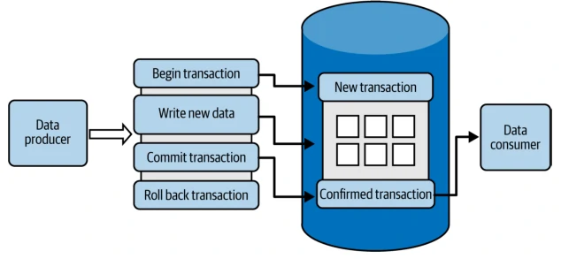
Transactions are another powerful database capability that can help us implement idempotent data producers. Transactions provide all-or-nothing semantics, where changes are fully visible to consumers only when the writer confirms them. This confirmation step is more commonly known as commit.

The best way to protect our consumers from the incomplete data issue is to leverage the transactions with the Transactional Writer pattern. It relies on the native database transactional capacity so that any of the in-progress but not committed changes will not be visible to downstream readers.

Workflow
- The producer initializes the transaction.
  - In the explicit mode, we need to call a transaction initialization instruction, such as START TRANSACTION or BEGIN.
  - In the implicit mode, our data processing layer handles the transaction opening on our behalf.
- Write the data.
  - The changes are added to the database but remain private to our transaction scope.
- Commit
  - When we have finished writing the data, do we need to change the new records’ visibility to make them publicly available to consumers.
  - If there is an issue, instead of publishing the data, we need to discard it by calling the action that is the opposite of the commit step, which is rollback.
  - From a low-level point of view, there are two implementations that we will use, depending on our processing model.
    - Standalone jobs or ELT workloads processing datasets at the data storage layer (e.g. BigQuery, Redshift, or Snowflake). The transaction is usually declarative and fully managed by the data store, and the processing can be distributed.
    - Multiple tasks work in parallel to write a dataset to the same output.
    - The transaction is local (i.e., task based). Each task performs an isolated transaction. This works well as long as we don’t encounter any job retries.
    - The whole job is transactional. In this mode, the job initializes the transaction before it starts running the tasks, and it commits the transaction once all the tasks complete their work. This provides a stronger guarantee than the local transaction but is also more challenging to achieve.

The idempotency comes from the all-or-nothing transactions semantics. In case of any error, the producer doesn’t commit the transaction, which leads to either an automatic rollback or orphan records in the data storage layer that are not visible to the readers.

Consequences
- Commit step
  - Unlike a nontransactional write, a transactional one involves two extra steps, which are opening and committing the transaction, alongside resolving data conflicts at both stages. The steps may have an impact on the overall data availability latency.
- Distributed processing
  - Distributed data processing frameworks’ support for transactions is not global.
- Idempotency scope
  - the idempotency is limited to the transaction itself. if a distributed data processing framework uses local (i.e., task-based) transactions without any further coordination to store already committed tasks, any job restart will rewrite the data from committed transactions.
Example
- Modern table file formats (Delta Lake, Apache Iceberg, and Apache Hudi)
- Streaming brokers (Apache Kafka)
- Data warehouses (AWS Redshift and GCP BigQuery)
- Relational database management systems (PostgreSQL, MySQL, Oracle, and SQL Server).

Immutable Dataset

Proxy

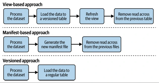
Case: We need to rework the pipeline to keep each copy but expose only the most recent table from a single place. The requirement expects the dataset to be immutable and thus written only once. To achieve this, we can implement the Proxy pattern.

Workflow
- We must guarantee the immutability by loading the new data into a different location each time. A good and easy solution is to use time-stamped or versioned tables. Their names are suffixed with a version or a timestamp to distinguish them. To keep the immutability, all writing permissions should be removed from these tables after creating them. Than, they will be writable only once. Another alternative is using storage layer, where we could enhance the access controls with a locking mechanism write once read many (WORM).
- Create a single data access point, which is the proxy. It’ll be a passthrough view that exposes the most recent table without any data transformations in the SELECT statement. If our data store doesn’t support a specific view, we’ll have to create a similar structure on our own.
Consequences
- Database support
  - Not all databases have this great view feature, which will be an immutable access point to expose underlying changing datasets. Although it can be replaced with a manifest file.
- Immutability configuration
  - We can enforce immutability at the data orchestration level by configuring the output of the triggered writing task.
Examples
- Apache Airflow + PostgreSQL: loading the data into a hidden internal table COPY command. CREATE OR REPLACE VIEW command for refresh view and write the new dataset to a different table.

Data Value

Data value design patterns purpose is to augment the dataset to improve its usefulness for end users.

Data Enrichment

Raw data will be poor because of technical constraints. Data enrichment patterns overcome this limitation and make data more useful.

Static Joiner

Enrich dataset using static reference dataset. The at-rest character of the joined dataset presents the perfect condition for using the Static Joiner pattern. The pattern also works for streaming pipelines.

The implementation requires a list of attributes from both datasets that may be used to combine the datasets.

Besides this keyed condition, the combination may also expect some time constraints, especially when the enrichment dataset implements some form of slowly changing dimensions. In that case, we could implement a time-sensitive static joiner variation of the initial pattern.

Example
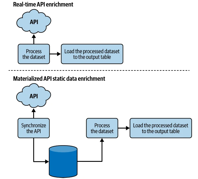
- SQL + SCD table: JOIN statement.
- Programmatic API: direct process, materialized API data.
- Programmatic API + idempotency: materialized API data.
- Apache Spark + API: Stream-to-batch join. .join operation.

drawing

Consequences
- Late data and consistency
  - In an ideal scenario, the data would evolve at the same pace as events are produced. But with late data, this scenario needs to mitigate. To mitigate the latency issue in streaming pipelines, we can use the Dynamic Joiner pattern.
  - It considers the enrichment dataset to be a dynamic one and uses adapted join conditions in that context. The mitigation is simpler for batch pipelines, where we can rely on the orchestration to wait for the enrichment dataset to be present.
- Idempotency
  - If we backfill a batch pipeline, we should ask ourself whether the outcome must be idempotent for the enrichment dataset. If that’s the case we may need to bring the enrichment dataset into our data layer to control the time aspects before doing the join.
  - The situation is even trickier when it comes to the external datasets hidden behind an API. Here too, ideally, we should be able to issue time-based queries, but this may not be possible. The solution could be adding this temporality into our internal data store and writing all enrichment records there.

Dynamic Joiner

The Static Joiner pattern isn’t the best fit for combining two streaming datasets. The problem lies in the data perception. Streaming stands for a continuously moving dataset, with as-soon-aspossible processing, while static batch workloads operate on more slowly evolving data.

The Dynamic Joiner pattern, which is better suited for that kind of data as both datasets are in motion.

The implementation shares some points with the Static Joiner, the identification of the keys and the definition of the join method—there is one extra requirement: time boundaries. Without this dedicated time management strategy, there’s a risk that many of the joins will be empty. It’s simply because the two datasets may have different latencies. The enrichment dataset can be late compared with the enriched dataset or vice versa. To mitigate this issue, dynamic joins are often completed with additional time conditions.

Defining these time conditions implies having a time-bounded buffer for joined records on both streams. The faster data source can align its time semantics with the slower data source. The buffer gives some extra time for joins to happen. This extra time is often an allowed latency difference between the data sources.

The buffer involves a streaming aspect called the garbage collection (GC) watermark. Even though technically, we can always decide to keep events from both streams forever, this will require significant hardware resources and will fail sooner or later if we cannot scale our infrastructure indefinitely. A better approach is to define when events that are too old should go away from each buffer, meaning when we should use a GC watermark. This obviously means losing the join if one of the records comes really late, but that’s the tradeoff for having a manageable size buffer.

drawing

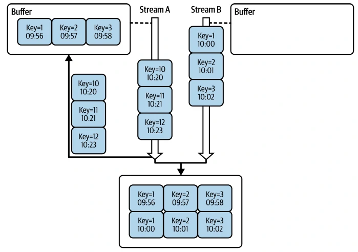
Due to the difference, to maximize the success rate of the joined records, Stream A buffers all unmatched keys for a period time. Then, when Stream B catches up, Stream A tries to find the corresponding rows either from the incoming data or directly from the buffer. If there is no match, the GC watermark removes records that are older than Stream B’s oldest event time.

Consequences
- Space versus exactness trade-off
  - Due to the GC watermark and time boundaries, we may not be able to get all the joins that are possible. We can optimize efficency by increasing buffer space, but it’ll cost us more hardware resources. On the other hand, reducing space optimizes storage but may reduce the likelihood of matching if the latency difference is too big.
- Late data
  - Late data is another reason for missed joins. Stream processing, due to its inherently lower latency processing semantics, has a weaker tolerance for late data integration in the pipelines.

But neither of the two data enrichment patterns presented here will give us a 100% guarantee of the join results without any extra effort, due to this late data arrival issue.

Example
- Apache Spark: .join operation + withWatermark expression.
- Apache Flink: temporal table joins.

Data Decoration

Wrapper

Wrapping consists of adding an extra behavior or attribute(s) to an object. It also helps separate the original parts of a record from transformed parts.

The process here is to clearly separate the computed values from the original ones to simplify processing logic but keep the original structure for debugging needs.

The idea is to add an extra abstraction at the record’s level. The abstraction wraps the original values with a high-level envelope. In addition to these initial attributes, the envelope references computed attributes that may come from the input data itself or from the execution context.

A design pattern that encapsulates an original data record inside another structure while attaching additional metadata, computed attributes, execution context, processing state, or governance information, without mutating the original record.

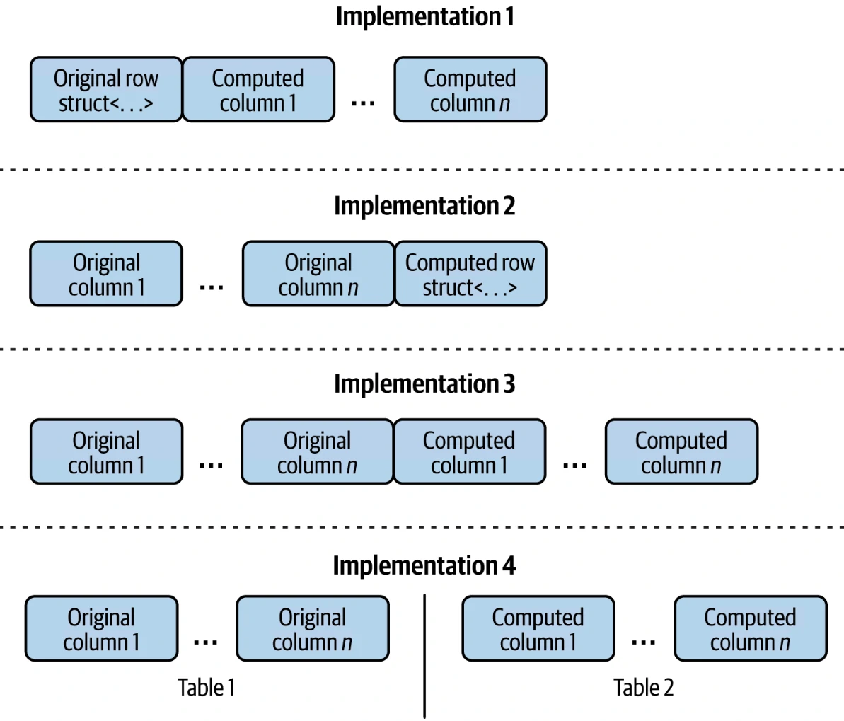
There are four different wrapping implementations for structured data:
- Implementation 1 stores the original row in a flat structure and all computed columns as nested attributes.
- Implementation 2 does the opposite (i.e., it stores computed rows as a single flat structure).
- Implementation 3 stores all columns in a flat structure at the same level.
- Implementation 4 stores the data in two separate tables that can be joined later by a unique key.

The first two implementations use a denormalization approach that may be faster at reading. The third one uses the normalized approach, which may be slower at reading but can be a better choice if we need to logically isolate the datasets or when we simply can’t change the original structure.

drawing

Consequences
- Domain split
  - This is the logical implication because the pattern divides attributes for a given domain.
  - If we implement the Wrapper, we’ll find user-related fields in two different high-level structures: raw and computed. Although this approach has some advantages, such as making a clear distinction between transformed and nontransformed values, it also makes data retrieval more complicated.
  - As a trade-off, we could consider the wrapped data to be the data belonging to the first storage layers of our system, like the Silver layer from our use case, and not the final data exposed to the users, for whom this separation may be confusing.
- Size
  - Decorated values form an intrinsic part of the processed record, and therefore, they impact the overall size and network traffic. When it comes to the size impact in the Wrapper pattern, we can mitigate the limitations if our data storage format supports data source projection. With this feature, we can select the columns we are interested in and ask the data source to physically access only them.
Example
- Apache Spark + PySpark API: wrapping operation.
- Apache Spark + SQL: decorated operation. (e.g. NAMED_STRUCT function).

Case

Original

data
---------
customer_id
age
order
---------

{
"customer_id": 1001,
"age": 22,
"order": 6000
}

Original + Transform

folder
----------------------
Average = 88
Grade = A
Rank = 5
Comment = Excellent
----------------------
Original Report Card
----------------------
customer_id
age
order
----------------------

{
    "original":{
        "customer_id":1001,
        "age":22,
        "salary":6000
    },

    "computed":{
        "risk_score":0.72,
        "segment":"Gold",
        "fraud_probability":0.02
    },

    "metadata":{
        "quality_score":98,
        "pipeline":"CustomerRiskV3",
        "processing_time":"2026-07-23"
    }
}

Architecture

              Source Record
                    │
                    ▼
          Wrapper / Envelope
  ┌───────────────────────────┐
  │ Metadata                  │
  │ Computed Attributes       │
  │ Processing Context        │
  │ Lineage                   │
  │ Validation Results        │
  │                           │
  │     Original Record       │
  └───────────────────────────┘

Core Components

  Envelope
    ├── Original Data
    ├── Derived Data
    ├── Metadata
    ├── Processing Context
    ├── Validation
    ├── Audit
    └── Lineage

Metadata Decorator

This process is needs for hide the extra records in the metadata layer of our data store.

For example, in actively evolve process, we need some visibility into thei mpact of the released version on the generated data. To simplify our maintenance activity, we need to add some technical context to each generated record, such as the job version.

Including the technical context in the record with the Wrapper pattern is not an option here. This information may not be relevant to our consumers since they’re not interested in our internal data processing details. Instead, we can leverage the metadata layer of our data store to apply the Metadata Decorator pattern.

The implementation will depend on our data store capabilities for handling metadata. If it supports the metadata out of the box, we will be able to associate each written record with a dedicated metadata attribute. Since this attribute is a native part of the data producer’s capabilities, the implementation is relatively straightforward.

Example
- Apache Kafka: list of optional header key-value pairs. includeHeaders command.
- Common object stores: define the metadata attributes as tags
- Relational or NoSQL databases: Simulate the decoration by including the metadata within the data part but without publicly exposing it to end users. (E.g. a column processing_context with value {"job_version”: “v1.0.3”, “processing_time”:"2023-06-10T10:02:00Z"})
- Relational or NoSQL databases: store the processing context in a dedicated table
Consequences
- Implementation
  - Implementation can also be challenging for table datasets, where, as demonstrated before, we’ll often need to define an extra column or table to handle the metadata information. Although this works, it requires more effort than for data stores that natively support metadata decoration.
- Data
  - Even though there is no technical limitation on what type of information we can put into the metadata layer, we should avoid writing business-related attributes there, such as shipment addresses or invoice amounts.

Data Aggregation

Distributed Aggregator

Case
- Building an online analytical processing (OLAP) cube, thereby reducing all data to an aggregated format that’s well suited to our dash boarding scenarios. The result should include basic statistics (count, average duration, etc.) across multiple axes (user geography, devices, etc.).
- The dataset is stored in daily event time partitions, and the analytics cubes should represent daily and weekly views.
- The Distributed Aggregator pattern leverages multiple machines that together form a single execution unit called a cluster. These servers individually don’t have enough capacity to process the whole input dataset, but together, they divide the work and can handle this scenario.
- Execution of the Distributed Aggregator involves a step to exchange records that were initially loaded into different machines, across the network. As a result, the reduce function can operate on all necessary collocated rows. The action depicted is called a shuffle. Often, it is one of the first latency trouble‐ makers because of the network traffic cost.
Consequences
- Additional network exchange
  - The pattern involves two network exchanges.
  - The first brings input data to each node.
  - The second network exchange comes from the Distributed Aggregator pattern because it’s a required step to gather related data on the same server. This is one of the possible latency issues to look at when problems arise.
- Data skew
  - With unbalanced distribution dataset, the cost of moving it across the network and processing it in a single node will be the highest.
  - Some techniques exist to prevent the skew, such as salting, which consists of adding an extra value (aka salt) to the grouping key and performing the first grouping operation on the salted column.
  - Next, if we need to get the results for the original grouping key, we’ll need to aggregate the outcome of the salted column’s aggregation again.
- Scaling
  - A node has completed all planned reduce opera‐ tions, it may still be in use by the hardware layer for fault tolerance reasons.
  - If the whole reduce computation fails and gets restarted, this data won’t need to be reshuffled again—but when there is no failure, the node will still be there but will not be reclaimed as long as the processing is running. If we want to avoid keeping it for all that time, we can opt for a component called shuffle service.
  - Shuffle service is an additional compute component that is responsible for storing and serving only shuffle data.
Example
- Spache Spark + PostgreSQL + JSON: Exchange hashpartitioning node
- GCP BigQuery: Google Cloud Storage (GCS) service + external table

Local Aggregator

We have a streaming job that generates windows for data in a partitioned streaming broker. The data volume is static, and we don’t expect any sudden variations or changes in the underlying partitioning. As a result, the partitions number will never change.

On the surface, the Local Aggregator pattern still performs some aggregations, it does so locally with the single network exchange of reading the input data. This solution works thanks to the fixed partitioning schema and correct input data distribution. All records that are relevant for a given grouping key are already present in the same input partition, so there’s no need to load them from other places.

Advantage
- The lack of shuffle
- Fully isolated: meaning they won’t need to wait for the data on other tasks and can move forward.

The implementation effort should focus here on the producer side. It must guarantee to write a record with a particular grouping key to the same physical partition. On the consumer side, some of the tools provide facility methods to adapt the prepartitioned dataset to its shuffle format.

Example
- Kafka Streams: groupByKey method
- pache Spark: per-partition operations, such as mapPartitions and foreach Partition.

The logic we’ve just presented applies to the partitioned data sources whose volume is too big to be processed in a single machine. However, if we are working on a non-partitioned or partitioned but small dataset, we don’t need to worry about static numbers of partitions.

Consequences
- Scaling
  - Scaling is the most visible issue. The pattern depends on the static nature of the data source and consistent partitioning. If we can’t guarantee one of these conditions (e.g. given key will always be available from only one processing partition), the pattern won’t work correctly because it’ll create one or multiple groups for a given key whenever we change storage partitions.
  - For scaling, we could do it with a dedicated data storage reorganization task, which would regenerate the partition assignments for all the records.
- Grouping keys
  - For partitioned data sources with static numbers of partitions, the pattern also expects one grouping key logic for all consumers.
  - It would involve writing the same record in multiple places, each time with a different grouping key.

Sessionization

Sessions are special kinds of aggregators since they combine events related to the same activity. In each of the activities, we create a session composed of a starting point, session events, and an ending point.

Incremental Sessionizer

A session sounds like a real-time component, but the generation method also supports batch processing.

Cases We records visit events in an hourly partitioned location, thus for one session may be present in multiple consecutive partitions, the problem belongs to the incremental processing family. To solve it, we can leverage the Incremental Sessionizer pattern.

The implementation requires setting up the following three storage spaces:
- Input dataset storage: This stores the raw events we need to correlate in the sessionization pipeline. There, we’ll find the hourly partitioned visits from the problem statement.
- Completed sessions storage: This is the place where we’ll write all finished sessions. Eventually, we could also write the ongoing sessions here as well, but ideally, we should distinguish them from the completed sessions (e.g. add atribute like is_final set to false whenever a session is still active).
- Pending sessions storage: Store all sessions spread across multiple partitions that will be closed in one of the next executions. There are two differences between this and completed sessions storage.
  - First, it must remain private and evolve with our internal logic. End users doesn’t need to be aware of the details, and if they were, we would have less evolution flexibility.
  - Second, the data format for the sessions can be different from the format in completed sessions storage. We could include some technical or internals details here, such as execution ID, if it would be helpful in defining the processing logic.
We also need to define the workflow logic. The logic starts by combining the input dataset with all pending sessions generated in the previous execution. The combination happens for each session entity—such as a user, product, or visit—and it can generate the following:
- A new session if there is no pending session for a given session entity.
- A restored session with new data coming from the read input.
- A restored session without new session data. This session will probably be about to expire in this or the next execution, depending on the expiration rules we ’ve defined.
Once we complete this combination, we’ll get session data to process, possibly composed of previous and new records. On top of that, we need to apply sessionization logic that defines three states:
- Initialization: When a session starts. For example, it can start when a particular event type occurs such as visiting the home page of our blog.
- Accumulation: When a session is live. What do we do with new incoming data? For example, we could store the visited pages in order.
- Finalization: When a session stops. A session can finish when a particular event type occurs or because of a period of inactivity.
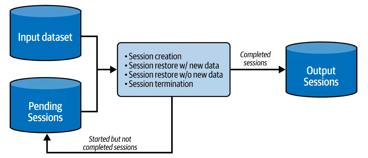
In the schema, we can see the execution flow with all involved storage spaces. The transformation loads pending sessions created in the previous run and new data available in the input dataset. Afterward, all completed sessions go into the publicly exposed storage while all pending sessions are written elsewhere to keep them alive and available for the next job execution.

Implement WINDOW function or a GROUP BY expression for processing logic.
Consequences
- Inactivity period
  - The inactivity period defines how long we can keep a session open. The longer it is, the more late data we can include in the session. But this will require more compute and storage resources to handle the late data.
  - We should find the right balance between the compute requirements and the business logic because it’ll be challenging to have both.
  - A long inactivity period threshold will also keep the sessions in the hidden space for that amount of time.
  - A partial session is not a completed session, and it may change in subsequent versions.
  - It’s therefore important to flag the ongoing sessions—for example, with an attribute like is_completed: false
- Data freshness
  - The Incremental Sessionizer works for batch pipelines, which are still the first choice of processing mode for data teams.
  - This will make the insights often come very late compared to real time.
  - To mitigate this issue and still be able to use batch pipelines, we can create the partial sessions introduced in the previous section.
- Late data, event time partitions, and backfilling
  - If our sessionization logic relies on event time partitioning, late data will be a problem as we may miss sessions for already processed partitions.
  - A session generated for the partition at 09:00 directly impacts the session at 10:00, the one at 10:00 impacts the one at 11:00, and so on.
  - This dependency is also visible in backfilling. If we rerun the session generation logic for one partition, we’ll have to do the same for all subsequent partitions. This can become expensive very quickly.
  - The simple solution of replaying all partitions after the backfilled one is easy for the code but costly.
  - On the other hand, having a smart detection method to find entities to backfill and rerunning only them from a dedicated backfill pipeline optimizes the cost but adds extra complexity.
Examples
- Apache Airflow: DELETE FROM statements -> runs the session generation query -> loads all input data into a temporary -> session-scoped visits table -> insert pending and finished.

Stateful Sessionizer

If data freshness is an issue, the Incremental Sessionizer will not help us. We should use another sessionization pattern that performs great on top of the stream processing layer, thanks to its more frequent and smaller iterations.

For need to access the session in a lower latency, it available in our streaming broker within seconds, although it need some modification that default streaming pipelines won’t help either because they are stateless.

Stateful pipelines bring an extra component called a state store. In our sessionization context, the state store plays the same role as the pending sessions storage zone in the Incremental Sessionizer.

But this storage for pending sessions is not the Stateful Sessionizer’s only similarity to the Incremental Sessionizer. The Stateful Sessionizer’s implementation follows the same workflow as for the Incremental Sessionizer:

Creating a session, or resuming the sessionizer.
Combines the created or resumed session with new incoming records according to our business logic.
If the session is completed or the partial sessions need to be available to consumers, the pattern transforms and writes the pending session record into the final output. Additionally, if the session is not completed, this step also writes the new state to the state store.

drawing

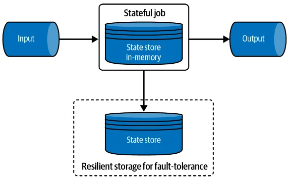
The schema illustrates the interaction between a stateful data processing job and its state store. There are two flavors of the store.

The first one is for fast access. It lives in memory, which of course involves volatility.
To overcome the risk of losing the state in case of failure or restart, the job synchronizes the state regularly to a more resilient fault tolerance storage.

The data processing logic can rely on the following data processing abstractions:

Session windows: a window created for each session key. Its length is specified by a gap duration, which is the maximum allowable period of inactivity between two events with the same session key before it creates a new session windows.
Arbitrary stateful processing: This approach requires more implementation effort but it also provides more flexibility.
Consequences
- At-least-once processing
  - Saving the state on fault tolerance storage doesn’t happen during every state update. Instead the writing process (checkpointing) occurs irregularly. Any stopped job restarts from the last successful checkpoint, leading to at-least-once processing.
- Scaling
  - Changing the compute capacity in this stateful context may involve state rebalancing. The job will not be able to process the data as long as the particular state keys are not assigned to new workers.
- Inactivity period length
  - Need to set the right balance to keep the total cost acceptable and include as many sessions as possible. That will impact to hardware pressure and output freshness.
- Inactivity period time
  - Besides emitting the sessions to the output storage, the solution will also need to manage the expiration of the state for all completed sessions. E.g. from incoming events and time-based expiration.
Examples:
- Apache Spark: stateful mapping function
- Apache Flink: VisitToSessionConverter convertor

Data Ordering

Bin Pack Orderer

One of the nightmares for ordered data delivery at scale is partial commits. E.g. from a bulk API to write multiple items and optimize network communication.

From events process, the data need to expose from an external API to external websites for analytics purposes. To optimize the cost, the job must be common for all consumers. It has to create a processing time window of 10 minutes with per-minute aggregates, and in the end, it must flush the buffer to different outputs provided by consumers. The events must be delivered individually for each minute and consumer, and in event time order.

We can solve the problem if we deliver each record individually. But, that implies significant network overhead as we’ll need to initialize as many requests as there are records. We can mitigate the issue by relying on the bulk operations that together with the Bin Pack Orderer pattern.

The implementation follows two important steps:

Responsible for grouping all related events and sorting them. The result will be records sorted within the same entity.
We need to pack those rows in bins individually. We create isolated subsets that we can deliver through a bulk API without worrying about completeness, duplicates, and partial commits.
Workflow
- Sorts the records by their grouping key and time
- The algorithm places the sorted rows into delivery bins so that there is only one grouping key in each bin. The bins can be arrays or lists.
- Emits bins sequentially.
  - It doesn’t interfere with the ordering for the retried grouping key. because there is only a single occurrence per bin.
  - The next bin isn’t delivered as long as the current one is not fully written to the output.
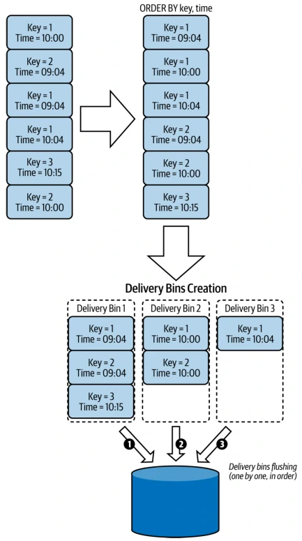
Consequences
- Retries
  - The pattern guarantees ordering inside the same execution.
  - If our whole pipeline fails, then the retry will involve already emitted results.
- Complexity
  - The bin packer is definitely more difficult to implement than a classical sort.
  - It requires a custom sorting and bin creation logic.
Examples
- Apache Spark: a local sorting mechanism + a local group by event_time.

FIFO Orderer

This pattern can be good for use cases that don’t require low latency or a large volume of data. Expecially the requirement is to deliver each record as soon as possible, so any buffering to optimize the network traffic is not an option.

Buffering and bulk requests help reduce network overhead in data transmission. However, in environments with more relaxed delivery constraints FIFO Orderer pattern will more suitable.

It doesn’t require any specific sorting algorithm since the requirement is to send data in the first in, first out (FIFO) manner. Instead, it only detects the records and issues the delivery request. An important thing is to get the delivery acknowledgment for each record before proceeding to the next one. Otherwise, it may lead to issues of data being out of order or lost.

Examples
- API delivering one record at a time
- a bulk API with concurrency 1 level
- Apache Kafka: produce(...) function + synchronous flush(...) invocation or producer delivers each record individually.
- Apache Kafka: for bulk requests, producer({max.in.flight.requests.per.connection})
Consequences
- I/O overhead and latency
  - Despite the possibility of using bulk API under some conditions in some data stores, is the I/O overhead and resulting increased latency as the data store and data producer must handle requests individually.
  - Instead of sending one network request for many records, the FIFO Orderer pattern sends one request for each input row.
  - Reduce this impact by leveraging multithreading, meaning by issuing the individual requests from multiple processes of our producer. The only problem is guaranteeing the ordering between these processes due to isolated and not aware of each other.
- FIFO is not exactly once
  - FIFO stands only for delivering the oldest records first, and it doesn’t guarantee the exactly-once delivery by itself. To mitigate this issue, we’ll need to rely on one of the idempotency patterns.

Data Flow Design

The goal of data flow design patterns is to design and coordinate all steps required to generate a dataset. This involves actions like chaining various tasks in a pipeline, creating parallel or exclusive execution branches, or even managing the dependency of physically separated pipelines.

Data flow design patterns operate at two different levels:

Data orchestration, where they work in one or many data pipelines. Design patterns useful when we want to address the cross-teams collaboration issue. This level can leverage to manage the concurrency of our pipelines.
Data processing layer, which is the environment of our job. Design patterns help to better organize business logic to make it more obvious and easier to maintain over time. With sequence patterns, we can coordinate tasks or pipelines within a single pipeline or across many pipelines.
Sequence

This is an important factor that will impact the complexity, performance, and maintenance of the pipelines. This pattern will address the issue when a data processing job writing the processed dataset to multiple places, but when we need to replay only the loading part for one of the database, it dont have to restart the whole execution.

Local Sequencer

It orchestrates tasks locally (i.e., within the same pipeline or data processing job).

The good engineering practice is:

To simplify complex logic consists of decomposing it into smaller and therefore more approachable steps
Reorganization improves readability
Highlights the separation of concerns

The end goal is to decouple one big component into multiple smaller but connected items that will be run sequentially. The dependency between tasks should be organized according to the dataset dependencies.

E.g. in Ingestion process, we should create two tasks: Readiness Marker pattern (to check the data), and full loeader pattern (to physically load the data). As image below, we can implement them either as dependent tasks (with data orchestration layer dependency) or as a single task (with data processing layer dependency).

drawing

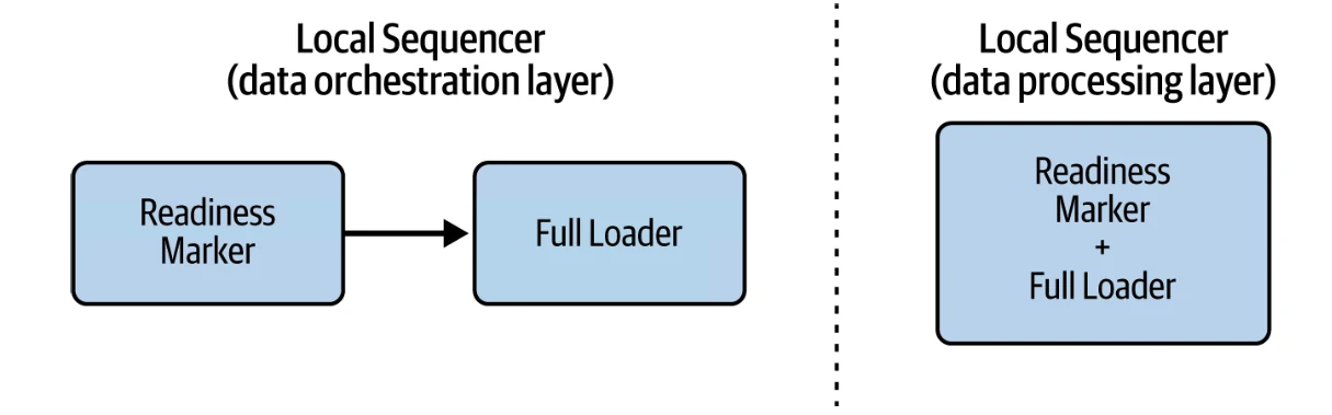
Criteria to decide whether the sequence should be based on the data orchestration layer or the data processing layer:

Separation of concerns: Putting all operations in the same item can make things harder to understand. A good indicator here is naming difficulty. If we struggle to find the name or if the name is too long in our opinion, this may be an indicator that we put too many operations into the single task on the data processing layer.
Maintainability: Relying on data processing sequentiality is also challenging for maintenance. In cases of backfilling or automatic retries, we will recompute all successful tasks prior to the failed one.
Implementation effort: The data orchestrator may provide different abstractions to perform common tasks out of the box, such as running a SQL query or executing an API call. If we combine all tasks into a single unit, we won’t be able to leverage this facility.
Consequences
- Boundaries
  - If we define boundaries incorrectly, execution time may grow too much or even impact other pipelines if we can’t scale the scheduler in our data orchestration logic. It’s therefore important to find a good balance between the scope and the number of tasks.
  - A good rule of thumb that applies to both the data processing layer and the data orchestration layer is to think about restart boundaries (i.e., what are the tasks that should be able to restart individually?). Thus the tasks should fail individually and shouldn’t impact each other and capable to restart individually.
  - Regarding the data processing job, we’ll often put the boundary between the most compute-expensive operations.
  - We can also reason for the logic separation in terms of transactions. If two or more operations must be performed as a single unit, it makes sense to keep them together.
Examples
- The data orchestration layer
  - Apache Airflow: Combining tasks consists of using the >> sign to express the dependency because the left side must run before the right one.
- The data processing level
  - SQL
  - API: python and Pyspark
  - The idea here is to consider each previously defined variable as an input for the next step, until we reach the data writing stage.

Isolated Sequencer

There is needs to not include the dashboards dataset transformation directly in our data preparation pipeline. The data visualization team asked us to provide the cleansed and enriched dataset only. The data visualization team will handle the transformation on its own.

The problem statement introduces two pipelines where one provides data to another. The objective here is to find a way to combine physically isolated pipelines. As with the Local Sequencer, the most important concern is the identification of boundaries.

The easiest solution consists of dividing the pipeline in terms of consumers and providers, or teams. If our team provides the dataset to a different team, then naturally, we can draw a boundary to create two isolated pipelines.

We may also face a situation in which we are the provider and a consumer at the same time. This may happen when the processed dataset is used by other pipelines within our team’s scope to generate other datasets.

How to do it:

To define boundaries in that context, we can analyze the complexity of the pipeline.
Finding the triggering mechanism. There are two strategies here: data based and task based.
- The data-based strategy is based on the Readiness Marker pattern. The data producer generates the dataset and a marker file to indicate it’s ready for processing. The consumer listens for this marker file and starts the work as soon as it detects the creation.
- The task-based strategy, the data producer doesn’t create a marker file. Instead, it directly triggers the pipeline responsible for consuming the generated dataset.

The two approaches have different couplings and shared responsibilities:

Pipelines from the data-based solution are loosely coupled. The only requirement is to respect the marker file.
The pipelines that form the task-based solution are tightly coupled. This means that, albeit physically separated, they can’t live alone.
In the data-based approach, the dataset consumer has more freedom. It can even decide to use a different dataset without notifying the data provider.
the task-based strategy, the consumer can’t simply decide to skip the dataset as the producer has the direct trigger mechanism.

drawing

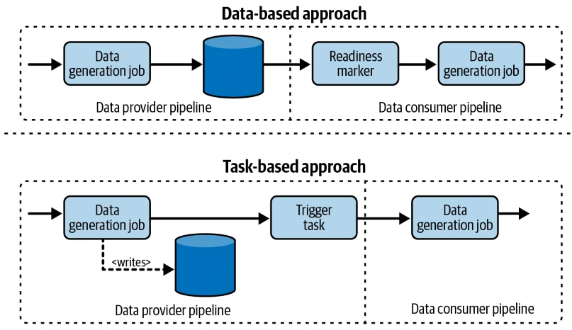
Consequences
- Scheduling
  - The task-based solution doesn’t impact just the evolution part. It is the scheduling frequency. The two pipelines should share the same schedule so that the producer can directly trigger the consumer. If that’s not the case, one of them will need to introduce more complexity.
  - If it’s the producer, it will need to add a condition to skip the triggering part for some of the planned execution schedules.
  - If it’s the consumer, it’ll have to do the same but by adapting its schedule to the producer and running the pysical data processing only when needed.
- Communication
  - The Isolated Sequencer addresses pipelines managed by different teams, among other things and need a good communication culture.
  - Either as a producer or as a consumer, we can add a mechanism that checks if the condition on the other side didn’t change.
Examples
- Apache Airflow

Data Design Pattern

Schema

Data Ingestion Design Patterns

Full Load

Pass-through Jobs

Incremental Load

Incremental Loader

Change Data Capture

Replication

Passthrough Replicator

Transformation Replicator

Data Compaction

Compactor

Data Readiness

Readiness Marker

Event Driven

External Trigger

Error Management Design Patterns

Unprocessable Records

Dead-Letter

Duplicated Records

Windowed Deduplicator

Late Data

Late Data Detector

Static Late Data Integrator (Circuit Breaker / CQRS)

Dynamic Late Data Integrator

Filter

Filter Interceptor

Fault Tolerance

Checkpointer

Idempotency Design Patterns

Overwriting

Fast Metadata Cleaner

Data Overwrite

Updates

Merger

Stateful Merger

Database

Keyed Idempotency

Transactional Writer

Immutable Dataset

Proxy

Data Value

Data Enrichment

Static Joiner

Dynamic Joiner

Data Decoration

Wrapper

Metadata Decorator

Data Aggregation

Distributed Aggregator

Local Aggregator

Sessionization

Incremental Sessionizer

Stateful Sessionizer

Data Ordering

Bin Pack Orderer

FIFO Orderer

Data Flow Design

Sequence

Local Sequencer

Isolated Sequencer