Land Change Detection (Encroachment Detection)
Computer Vision
Change Detection
Introduction
Operational assets are situated within highly dynamic environments where land use and land cover continuously evolve. Activities such as deforestation, urban expansion, erosion, land conversion, and unauthorized land occupation can significantly impact asset integrity, regulatory compliance, operational continuity, and environmental sustainability commitments.
Conventional monitoring approaches primarily rely on periodic field inspections and manual interpretation of aerial or drone imagery. While these methods provide valuable information, they are often time-consuming, resource-intensive, and reactive, limiting the ability to detect and respond to environmental changes promptly.
As regulatory requirements become more stringent and organizations strengthen their Environmental, Social, and Governance (ESG) commitments, there is an increasing need for a scalable, data-driven monitoring solution capable of continuously analyzing land use and land cover changes surrounding operational assets.
Business Challenges
Based on stakeholder assessments and detailed discussions, several key challenges have been identified in the current asset monitoring process:
- Manual Asset Monitoring: Asset condition monitoring is still largely dependent on traditional approaches, including periodic field inspections and manual analysis of drone imagery. The absence of an automated monitoring workflow leads to higher operational costs, longer inspection cycles, and increased potential for human error.
- Limited Visibility of Temporal Changes: Monitoring and understanding land use changes over time remains challenging, particularly across extensive and geographically dispersed operational areas. This limits the ability to identify gradual or emerging environmental changes that may affect asset performance.
- Delayed Detection of Encroachment Risks: Identifying unauthorized land use, encroachment, and other potentially harmful activities around operational assets is often delayed, reducing the organization’s ability to respond proactively and mitigate associated operational or legal risks.
- Lack of an Integrated Geospatial Monitoring Platform: The current monitoring process lacks an integrated Geographic Information System (GIS) capable of continuously detecting, analyzing, and visualizing land cover changes. This limits decision-makers’ ability to access timely, accurate, and actionable geospatial insights for effective asset management.
Goals
By integrating geospatial data, remote sensing technologies, and AI-driven analytics, the platform provides comprehensive situational awareness to support faster, more informed decision-making.
-
Centralized Geospatial Data Management: The Platform serves as a centralized repository for spatial data from multiple sources, including satellite imagery, drone surveys, GIS datasets, and field inspection records. By consolidating these datasets into a single, unified platform, all stakeholders gain access to consistent, accurate, and up-to-date geospatial information, improving collaboration and operational efficiency.
-
AI-Powered Change Detection Leveraging Image Analysis and Deep Learning capabilities, the solution automatically detects and analyzes land cover and land use changes around operational assets. Automated image processing significantly reduces manual interpretation, accelerates anomaly detection, and enables early identification of potential risks such as encroachment, deforestation, erosion, and unauthorized land activities.
-
Actionable Insights for Proactive Decision-Making: Geospatial intelligence is delivered through interactive dashboards, real-time maps, and analytical reports that provide clear visibility into asset conditions and environmental changes. These insights enable management teams to identify emerging risks earlier, prioritize response efforts, and make proactive decisions that minimize operational disruptions and reduce potential financial losses.
-
Enabling Sustainable Asset and Risk Management: By continuously monitoring asset surroundings through regularly updated geospatial data, the solution supports a proactive and sustainable approach to risk management. Organizations can monitor environmental changes, strengthen regulatory compliance, support ESG initiatives, and improve the resilience and continuity of operations across multiple locations.
Change Detection Framework
Methodology
Summarizes the required activities and the GeoAI strategy applied throughout the project.
The proposed land cover monitoring solution consists of four main stages: data preparation, model development, model deployment, and change detection. Together, these stages enable automated land cover classification and continuous monitoring of environmental changes around operational assets.
- Data Pre-processing: The pre-processing stage prepares high-quality datasets for developing a robust land cover classification model. This phase includes:
- Imagery Selection and Preparation – Collecting and selecting appropriate satellite or aerial imagery based on spatial resolution, acquisition date, and data quality.
- Image Pre-processing – Performing essential preprocessing tasks such as resampling, clipping to the area of interest, image alignment, reprojection, and quality enhancement to ensure dataset consistency.
- Dataset Finalization – Validating and organizing the processed imagery into a standardized dataset ready for model training.
- Ground Truth Labeling – Creating and validating object label polygons that represent land cover classes to serve as training labels for the deep learning model.
- Deep Learning Model Development: This stage focuses on building, training, and validating an AI model capable of accurately classifying land cover types.
- Training and Testing Dataset Preparation – Splitting labeled datasets into training and validation/testing subsets.
- Training Data Export – Preparing the labeled imagery in the required format for deep learning model training.
- Model Training – Training the deep learning model using the prepared datasets to learn land cover characteristics.
- Model Evaluation – Assessing model performance using validation data and evaluation metrics such as accuracy, precision, recall, F1-score, or Intersection over Union (IoU).
- Model Selection – Selecting the best-performing model for deployment based on evaluation results and operational requirements.
- Model Inference and Post-processing: After the model has been validated, it is deployed to classify land cover across operational areas beyond the training datasets.
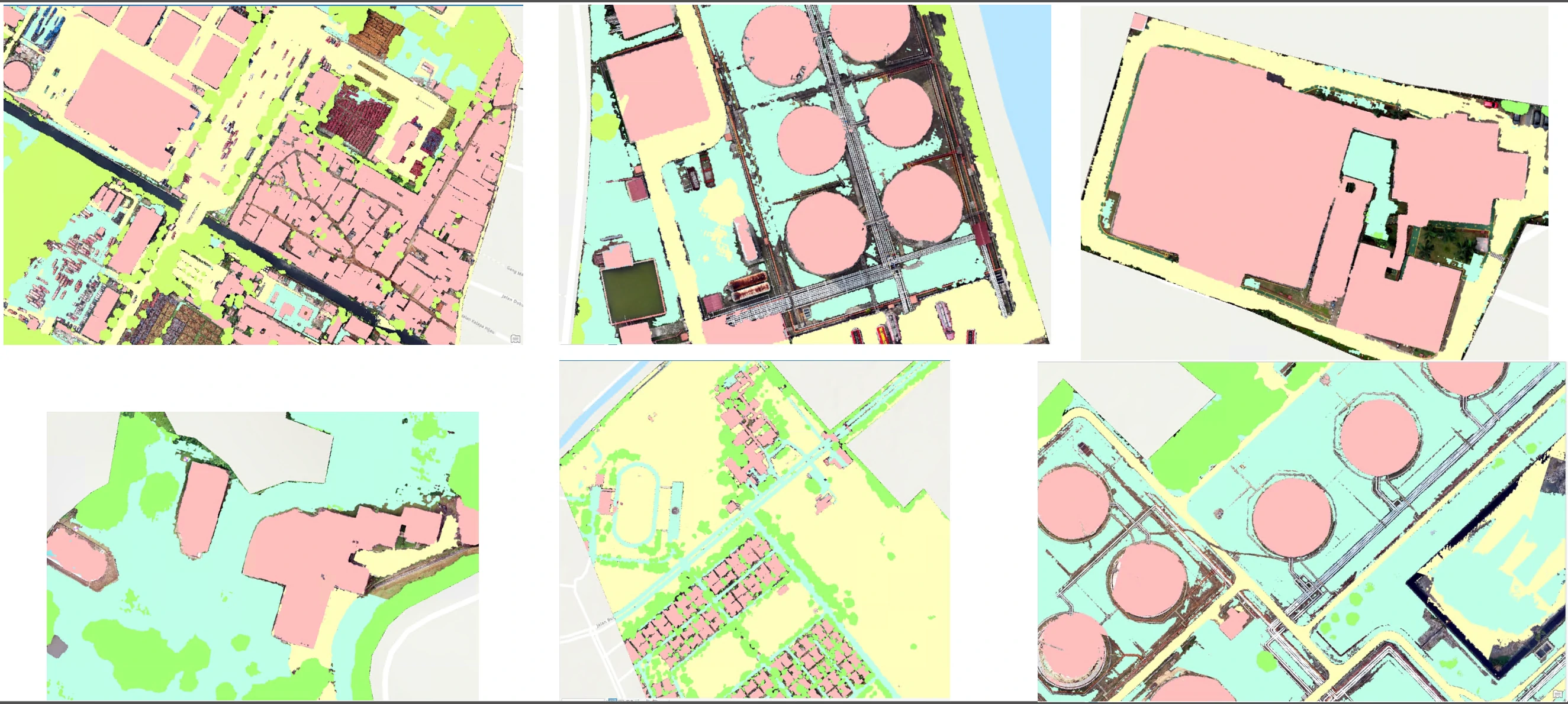
- Land Cover Prediction (Inference) – Applying the trained model to new satellite or aerial imagery to automatically generate land cover classifications.
- Post-processing – Converting raster prediction outputs into vector polygons, refining classification results, and preparing spatial datasets for visualization and further geospatial analysis.
- Land Cover Change Detection: The final stage identifies and quantifies land cover changes by comparing prediction results from different observation periods.
- Temporal Comparison – Comparing classified land cover maps from two or more time periods to identify spatial changes.
- Change Area Analysis – Calculating the extent and distribution of areas that have experienced land cover changes.
- Land Cover Transition Analysis – Identifying transitions between land cover classes (e.g., forest to bare land, vegetation to built-up area) to better understand the nature of the observed changes.
- Change Visualization – Presenting the detected changes through interactive GIS maps, thematic visualizations, and summary statistics, enabling stakeholders to quickly identify affected areas and support timely decision-making.
GeoAI Strategic

Data Assessment
Automated preprocessing
To minimize the risk of a “garbage-in, garbage-out” outcome, we conducted evaluations and adjustments
- Automated preprocessing that could be setup during acquisition process:
- Downscale resolution to 0.1m
- Standardize spatial references to WGS 1984 Web Mercator (Auxiliary Sphere)
- Standardize file name. File name will be parsed to get ID and time information.
- Selecting RGB band.
- Transform pixel depth to 8-bit.
- These steps help ensure that:
- Produces more reliable model outputs.
- Reduces load and improves processing time.
- Establishes a consistent baseline for improvement.
Manual preprocessing
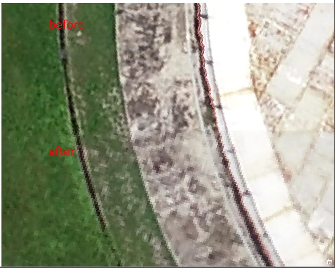
Manually fixing for shift due to difference Ground Control Point (GCP)
Manual preprocessing (non-automatable corrections):
- Image shifting caused by inconsistent Ground Control Points (GCPs)
- Misalignment leads to positional shifts that affect object boundaries and reference points.
- These shifts do not significantly impact land-cover classification but will directly affect any change-detection output.
Final Dataset Selection
Final Dataset Selection and Key Considerations
Based on the data assessments above, we propose the following dataset usage plan:
- Training and modeling dataset: 6 out of 12 datasets
- Excluded dataset: 1 out of 12 datasets (due to quality issues)
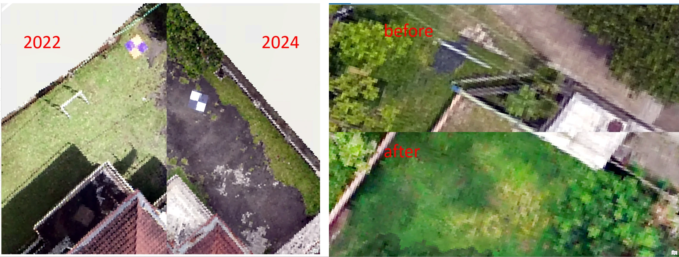
- GCP-shifted datasets: 3 out of 12 datasets
- These can still be used for GeoAI land-cover modeling.
- However, change-detection outputs from these datasets will be affected; objects will appear shifted and may be falsely classified as “changed.”
This distinction ensures reliable model performance while acknowledging the limitations for downstream change-detection analytics.
Labeling Strategy
Optimizing label quality is critical for improving model detection performance.
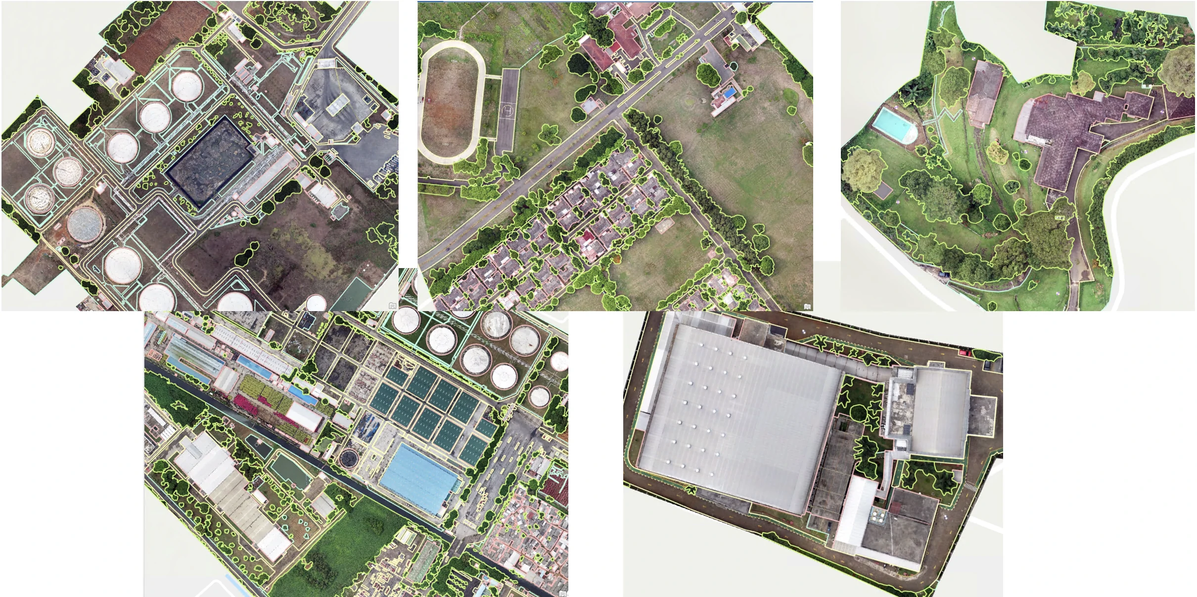
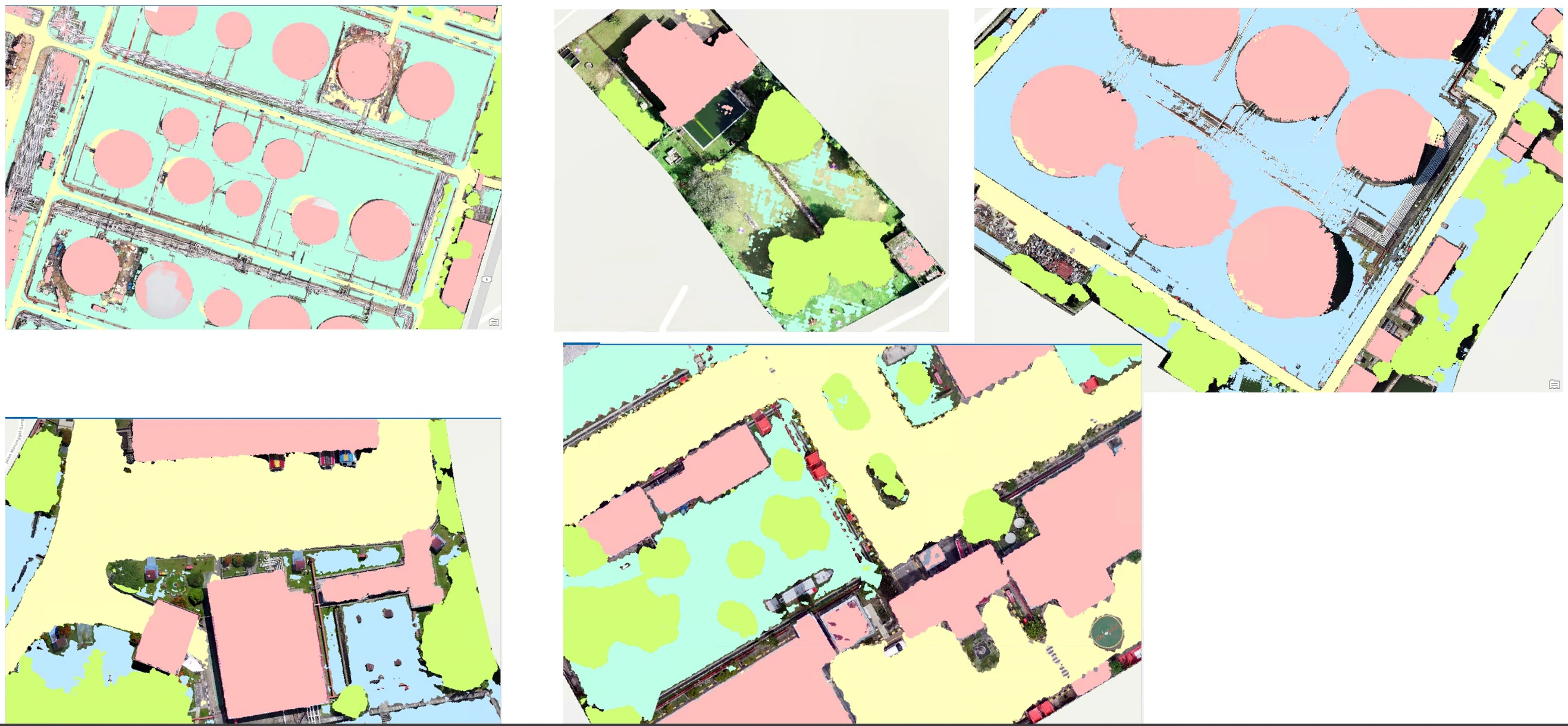
Following prior alignment discussions, we standardized the label schema into four target classes:
- Building – includes buildings, foundations, and cemented areas.
- Bareland – open land without significant objects.
- Street – roads not covered by trees; excludes small paths.
- Vegetation – large trees and tall plants; ornamental plants excluded.
All existing labels will be reprocessed and normalized to ensure consistency with this four-class standard and to maximize model accuracy.
Quantification of Label Data
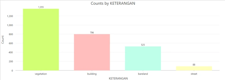
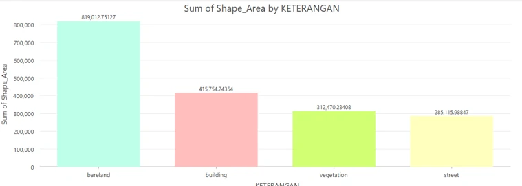
Quantification of label data; is relatively balanced across the four target classes.
For this iteration, we selected the most representative and cleanest subset of the available data (from the 12 total areas):
- 6 areas used for model training.
- 2764 total labeled objects.
- 1,832,351 m² total labeled area.
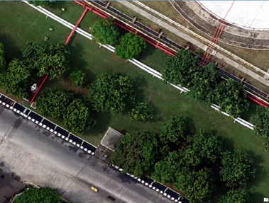
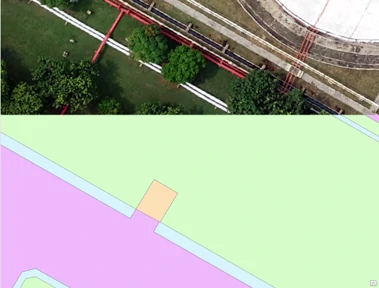
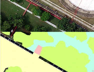
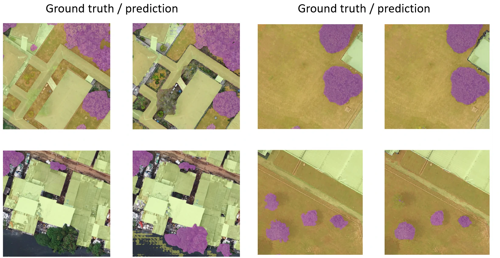
Samples of labeled data
Labeling Limitations
Labeling Limitations and Areas for Improvement
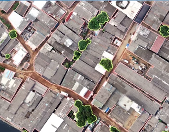
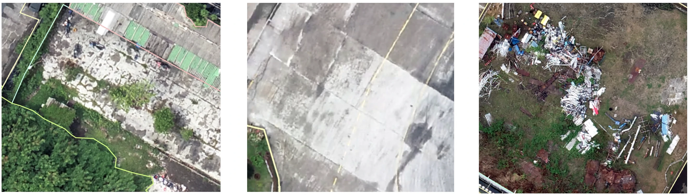
Certain land-cover elements share similar visual patterns, which may introduce ambiguities in the model’s predictions. Examples include:
- Streets and bareland sharing similar brown tones.
- Bareland with scattered small objects resembling building textures.
- Cement-layered streets appearing similar to building surfaces.
- Vegetation vs. bareland in areas with small or low vegetation, which is hard to distinguish from imagery alone.
For this project phase, our primary objective is encroachment detection, particularly identifying changes related to building labels. Thus, detecting the buildings will be prioritized and monitored on metrics and evaluation.
Modeling process
The model Architecture and the hardware that we used on training process.
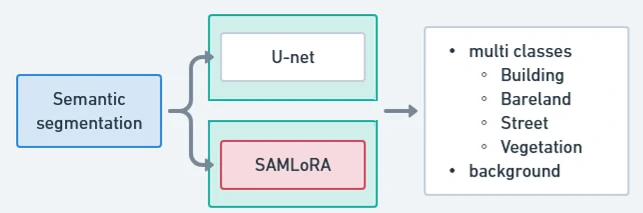
U-net: simple but powerful segmentation from scratch. SAMLoRA: Finetune model with prior knowledge.
Using internal GPU with these specification:
- NVIDIA RTX A2000
- VRAM: 12 GB
- Architecture: Ampere
- Memory interface: 192-bit
- Memory bandwidth: ~ 288 GB/s
- Tensor-Core peak: ~ 63.9 TFLOPS
- Using only dedicated memory without RAM included. It means the image will feed to GPU will be limited by its VRAM.
Training parameters:
- By only used dedicated memory, 2764 labels, and ~1.8M meter square area the images should have:
- 512 x 512 pixel per image
- Total images training= 3982 (996 for validation)
- Total Features= 29996
- Batch= 4
- Backbone: resnet 50 / resnet 101 for U-net and vit_l for SAMLoRA
Early Training Result
Summarize and determine how well our model learns from our dataset
Best combination (at early iteration):
- SAMLoRA with vit_l as backbone
- image size: 512
- Epoch: 32
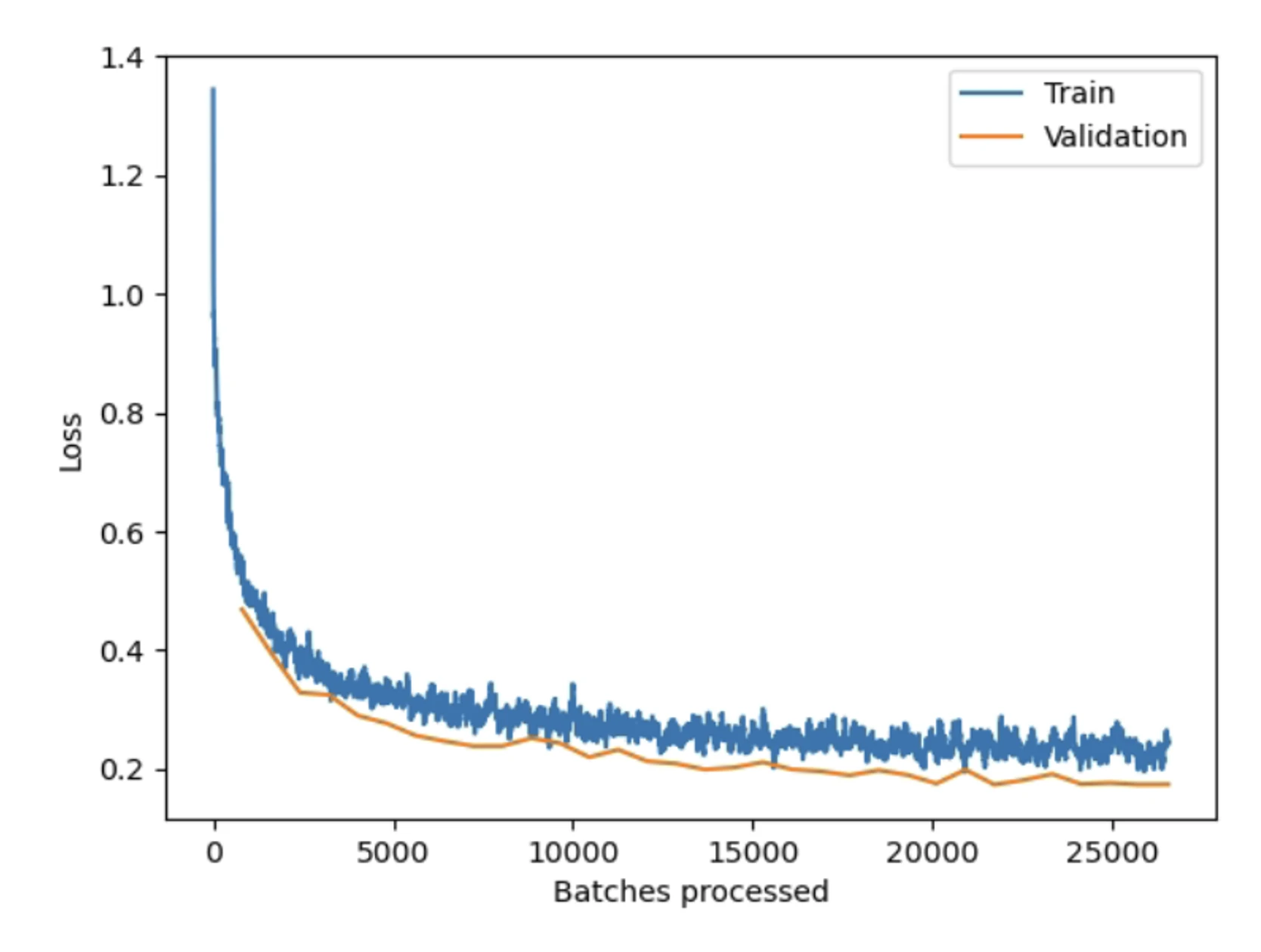
Evaluation matrics (Training process):
- Accuracy: 0.9079
- Dice: 0.8733
- Training time: 22:38:45
- Inference time: 0:27:54
| background | vegetation | street | bareland | building | |
|---|---|---|---|---|---|
| mIOU | 0.8190 | 0.8101 | 0.7926 | 0.8387 | 0.8843 |
| precision | 0.9078 | 0.9156 | 0.8557 | 0.8992 | 0.9556 |
| recall | 0.8932 | 0.8754 | 0.9149 | 0.92565 | 0.9221 |
| F1 | 0.9005 | 0.8951 | 0.8843 | 0.9122 | 0.9386 |
We propose to use dice and recall metrics for land cover model to determine how good our model compare to training, validating and testing data.
Early Testing result
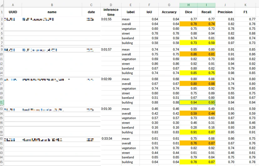
Result how well the model on unseen dataset
To ensure an unbiased assessment of model performance, we used a completely separate dataset for testing, to understanding of how the model will perform in operational conditions.
The results indicate:
- Strong performance in several areas.
- Opportunities for improvement.
These performance values are influenced by:
- Limitations in model,
- Labeling inconsistencies or ambiguities across datasets, and
- Variations in label quality for specific land-cover types.
Final Training Result
Best model:
- SAMLoRA with vit_l as backbone
- image size: 512
- rotation_angle: 90
- Epoch: 72
Evaluation matrics (Training process):
- Accuracy: 94.40%
- Dice: 92.01%
- Training time: 2 days, 5:10:58
- Inference time: 0:27:54
| background | vegetation | street | bareland | building | |
|---|---|---|---|---|---|
| mIOU | 88.79% | 85.32% | 88.07% | 89.84% | 93.68% |
| precision | 94.77% | 89.72% | 95.05% | 94.50% | 96.53% |
| recall | 93.36% | 94.55% | 92.30% | 94.80% | 96.94% |
| F1 | 94.06% | 92.07% | 93.65% | 94.65% | 96.73% |
Comparing result
Summarize and determine how well our best model compare to benchmark
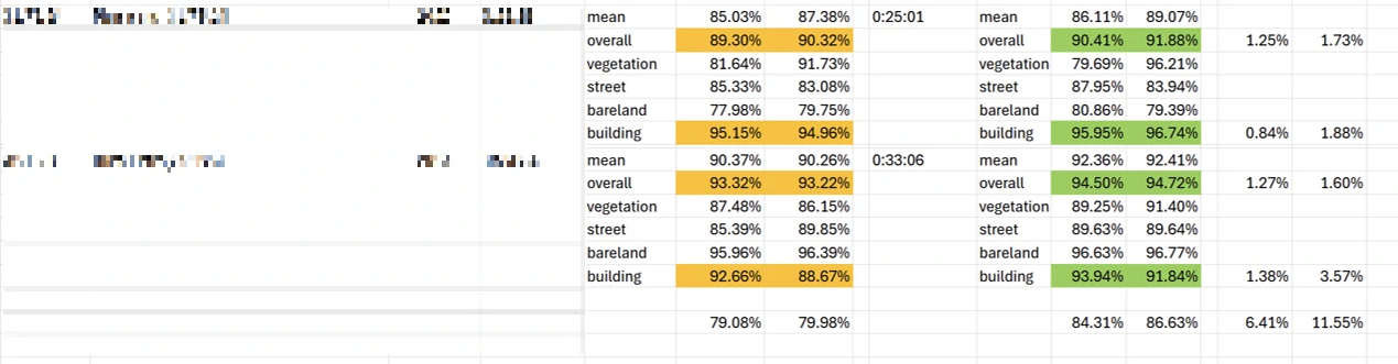
In our latest model release, performance metrics show a clear improvement compared to the previous benchmark reported in the last update.
The updated model demonstrates higher Dice and Recall scores across all tested areas. Minor reductions in certain measurements remain within our acceptable performance range.
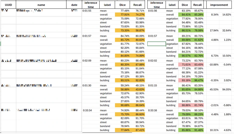
Overall, the new model achieves up to a 6.41% increase in Dice score and a 11.55% improvement in Recall, indicating a meaningful enhancement in segmentation accuracy and detection capability.