Multiple-criteria decision analysis (MCDA)
scoring
multiple-criteria
decision
Introduction
Multiple-criteria decision-making (MCDM) or multiple-criteria decision analysis (MCDA) is a sub-discipline of operations research that explicitly evaluates multiple conflicting criteria in decision making. It is also known as multi-attribute decision making (MADM), multiple attribute utility theory, multiple attribute value theory, multiple attribute preference theory, and multi-objective decision analysis.
MCDM is concerned with structuring and solving decision and planning problems involving multiple criteria. The purpose is to support decision-makers facing such problems. Typically, there does not exist a unique optimal solution for such problems and it is necessary to use decision-makers’ preferences to differentiate between solutions.
Solving can be interpreted in different ways. It could correspond to choosing the “best” alternative from a set of available alternatives (where best can be interpreted as the most preferred alternative of a decision-maker). Another interpretation of solving could be choosing a small set of good alternatives, or grouping alternatives into different preference sets. An extreme interpretation could be to find all efficient or nondominated alternatives.
Conceptual overview
Multi-criteria data are complex. This is because at least two syntactically disconnected vectors are needed to describe a problem.
- matrix /
Achoice set. The matrix must be a 2D array-like where every column is a criteria, and every row is an alternative. - And the vector of criteria optimality sense objectives /
C. Consider one attribute at a time and try to maximize or minimize it (as per the requirement) to generate optimized score. The objectives vector must be a 1D array-like with number of elements same as number of columns in the alternative matrix (matrix). Every component of the objectives vector represent the optimal sense of each criteria. - Additionally it can be accompanied by a vector w /
Wj with the weighting of the criteria to get optimized weighted scores. -
Combine the weighted scores (of each attribute) to create a final score for an entity.
- To make the data has same scale, and same target criteria. We will use two processors:
- First InvertMinimize which inverts the minimizing objectives. by dividing out the inverse of each criterion value (1/
Cj). - Second, SumScaler which will divide each criterion value by the total sum of the criteria, taking all of them into the range [0,1].
- First InvertMinimize which inverts the minimizing objectives. by dividing out the inverse of each criterion value (1/
- The first thing we must do now is to reverse the maximization criteria. This involves:
- Create the transformer and store it in the inverter variable.
- Apply the transformation by calling the transform method of the transformer and passing it as parameter our decision matrix dm.
- Save the transformed decision matrix in a new variable.
- The next step is to scale the values between using the SumScaler. For this step we need:
- Create the transformer and store it in the inverter variable. In this case the scalers support a parameter called target which can have three different values:
- target=”matrix” The matrix is normalized.
- target=”weights” normalizes the weights .
- target=”both” normalizes matrix and weights.
- In our case we are going to ask the scaler to scale both components of the decision matrix (target=”both”).
- Apply the transformation by calling the transform method of the transformer and passing it as parameter our decision matrix dmt.
- Save the transformed decision by overwriting the variable.
- Create the transformer and store it in the inverter variable. In this case the scalers support a parameter called target which can have three different values:
Algorithm
- Combined Compromise Solution (CoCoSo)
- The CoCoSo method combines the Weighted Sum Model (WSM) and Weighted Product Model (WPM) approaches to provide a comprehensive ranking solution for multi-criteria decision-making problems. It uses three different aggregation strategies to balance the advantages of both WSM and WPM methods.
- The method calculates three compromise scores:
- k_a: Arithmetic mean of normalized WSM and WPM scores
- k_b: Relative scores compared to the best alternatives
- k_c: Balanced compromise using the lambda parameter
- The final score combines these three measures using both geometric and arithmetic means to provide a robust ranking.
- Combinative Distance-Based Assessment - CODAS
- The CODAS method evaluates alternatives using two distance metrics.
- It first calculates both Euclidean and Taxicab distances from a negative-ideal solution, which represents the worst performance across all criteria.
- The method constructs a relative assessment matrix based on these distances, where the Euclidean distance serves as the primary measure, and the Taxicab distance acts as a tiebreaker when alternatives are very similar according to the first. The final ranking is determined by summing the values in the relative assessment matrix for each alternative, with higher scores indicating better performance.
- COPRAS (Complex Proportional Assessment)
- Is used to evaluate the superiority of one alternative over another. It supports comparison of alternatives based on maximizing and minimizing index values.
- Evaluation based on Distance from Average Solution - EDAS.
- The EDAS method evaluates alternatives by comparing them to an average solution benchmark.
- It calculates two key metrics: Positive Distance from Average (PDA) for performance exceeding the average, and Negative Distance from Average (NDA) for performance below average.
- These measures capture how each alternative deviates from the mean performance across all criteria.
- The final appraisal combines these deviations through a weighted, normalized scoring process. After computing weighted sums of PDA and NDA for each alternative, the method normalizes these values and averages them to produce a comprehensive evaluation score.
- ELimination Et Choix Traduisant la REalité - ELECTRE.
- Usually the ELECTRE Methods are used to discard some alternatives to the problem, which are unacceptable.
- After that we can use another MCDA to select the best one. The Advantage of using the Electre Methods before is that we can apply another MCDA with a restricted set of alternatives saving much time.
- Find a kernel of alternatives through ELECTRE-1.
- The ELECTRE I model find the kernel solution in a situation where true criteria and restricted outranking relations are given.
- That is, ELECTRE I cannot derive the ranking of alternatives but the kernel set. In ELECTRE I, two indices called the concordance index and the discordance index are used to measure the relations between objects
- Find the ranking solution through ELECTRE-2.
- To overcome ELECTRE I’s inability to produce a ranking of alternatives. Instead of simply finding the kernel set, ELECTRE II can order alternatives by introducing the strong and the weak outranking relations.
- Election based on Relative Value Distances (ERVD) decision-making
- This method integrates an s-shape value function, departing from the traditional expected utility function, to more accurately capture risk-averse and risk-seeking behaviors.
- ERVD builds upon the foundational principles of the TOPSIS method, extending its capabilities by incorporating concepts from prospect theory to refine the assessment of alternatives based on their relative distances from ideal and anti-ideal solutions.
- Multi-Attributive Border Approximation Area Comparison (MABAC)
- MABAC is a multi-criteria decision-making method that determines the distance of each alternative from the border approximation area. The method is based on the concept of border approximation area (BAA), which is calculated as the geometric mean of the weighted normalized decision matrix.
- The method consists of the following steps:
- Normalization of the decision matrix
- Calculation of the weighted normalized decision matrix
- Determination of the border approximation area (BAA)
- Calculation of the distance from BAA
- Calculation of the final score
- Multi-objective optimization on the basis of ratio analysis (MOORA)
- Ratio based MOORA method.
- In MOORA the set of ratios are suggested to be normalized as the square roots of the sum of squared responses as denominators, but you can use any scaler.
- These ratios, as dimensionless, seem to be the best choice among different ratios. These dimensionless ratios, situated between zero and one, are added in the case of maximization or subtracted in case of minimization
- Reference Point MOORA
- Rank the alternatives by distance to a reference point.
- The reference point is selected with the Min-Max Metric of Tchebycheff.
- This reference point theory starts from the already normalized ratios as suggested in the MOORA method.
- Preference is given to a reference point possessing as coordinates the dominating coordinates per attribute of the candidate alternatives and which is designated as the Maximal Objective Reference Point. This approach is called realistic and non-subjective as the coordinates, which are selected for the reference point, are realized in one of the candidate alternatives.
- Full Multiplicative Form
- Non-linear, non-additive ranking method method.
- Full Multiplicative Form does not use weights and does not require normalization.
- To combine a minimization and maximization of different criteria in the same problem all the method
- Combination of RatioMOORA, RefPointMOORA and FullMultiplicativeForm.
- These three methods represent all possible methods with dimensionless measures in multi-objective optimization and one can not argue that one method is better than or is of more importance than the others; so for determining the final ranking the implementation maximizes how many times an alternative i dominates and alternative j.
- Ratio based MOORA method.
- OCRA (Operational Competitiveness Rating)
- OCRA was initially intended to maximize the efficiency of a Production Unit (PU), seen as a set of activities that consume resources (inputs) and generate rewards (outputs), thus leading to a higher operational competitiveness.
- OCRA is thought of as an improvement of Data Envelopment Analysis (DEA): more efficient, robust, and properly sensitive to changes in inputs or outputs.
- In a general-purpose sense, PUs are the alternatives to be compared, and a quantity and value of each type of input/output is instead given as a criteria value and corresponding weight. Inputs are non-beneficial criteria that should be minimized, and Outputs are beneficial criteria that should be maximized; thus, the entire Decision Matrix is used.
- The performance of beneficial and non-beneficial criteria is computed separately and aggregated for each alternative, and then I/O criteria are summed to yield a final performance ranking.
- This means values are not scaled as 0-1 (possible future extension); however, they are floored to the Min value twice (first separately, then overall), such that the worst performance is always zero.
- PROBID (Preference Ranking On the Basis of Ideal-Average Distance) and SimplifiedPROBID (simple variation of PROBID).
- The distance metric to use If a string, the distance function can be braycurtis, canberra, chebyshev, cityblock, correlation, cosine, dice, euclidean, hamming, jaccard, jensenshannon, kulsinski, mahalanobis, matching, minkowski, rogerstanimoto, russellrao, seuclidean, sokalmichener, sokalsneath, sqeuclidean, wminkowski, yule.
- RAM (Root Assessment Method) decision-making
- RAM calculates the utility value of each alternative by aggregating their scores over the criteria, treating beneficial and non-beneficial criteria differently. The method uses an aggregation function that combines compensatory and partially compensatory characteristics.
- The weighted sum model (WSM)
- WSM is the best known and simplest multi-criteria decision analysis for evaluating a number of alternatives in terms of a number of decision criteria. It is very important to state here that it is applicable only when all the data are expressed in exactly the same unit.
- The weighted product model (WPM)
- WPM is a popular multi-criteria decision analysis method. It is similar to the weighted sum model. The main difference is that instead of addition in the main mathematical operation now there is multiplication.
- SIMUS (Sequential Interactive Model for Urban Systems)
- Is a tool to aid decision-making problems with multiple objectives. The method solves successive scenarios formulated as linear programs.
- For each scenario, the decision-maker must choose the criterion to be considered objective while the remaining restrictions constitute the constrains system that the projects are subject to.
- In each case, if there is a feasible solution that is optimum, it is recorded in a matrix of efficient results. Then, from this matrix two rankings allow the decision maker to compare results obtained by different procedures.
- The first ranking is obtained through a linear weighting of each column by a factor - equivalent of establishing a weight - and that measures the participation of the corresponding project. In the second ranking, the method uses dominance and subordinate relationships between projects, concepts from the French school of MCDM.
- The Stable Preference Ordering Towards Ideal Solution (SPOTIS)
- The SPOTIS method is a multi-criteria decision analysis method that is exempt of rank reversal. The method is rank reversal free because the preference ordering established from the score matrix of the MCDM problem does not require relative comparisons between the alternatives, but only comparisons with respect to the ideal solution (ISP) chosen by the MCDM designer.
- The Technique for Order of Preference by Similarity to Ideal Solution (TOPSIS)
- TOPSIS is based on the concept that the chosen alternative should have the shortest geometric distance from the ideal solution and the longest euclidean distance from the worst solution.
- An assumption of TOPSIS is that the criteria are monotonically increasing or decreasing, and also allow trade-offs between criteria, where a poor result in one criterion can be negated by a good result in another criterion.
- metric – The distance metric to use. If a string, the distance function can be braycurtis, canberra, chebyshev, cityblock, correlation, cosine, dice, euclidean, hamming, jaccard, jensenshannon, kulsinski, mahalanobis, matching, minkowski, rogerstanimoto, russellrao, seuclidean, sokalmichener, sokalsneath, sqeuclidean, wminkowski, yule.
- The VIKOR Method for Multi-Criteria Decision Making
- VIKOR (VIseKriterijumska Optimizacija I Kompromisno Resenje) introduces the concept of a compromise solution, which is a feasible solution that is closest to the ideal, and represents a balance between the majority rule (group utility) and the individual regret of the opponent.
- The method evaluates alternatives by converting an n-criteria decision problem into a bi-criteria one using the Manhattan distance (Sk, or group utility) and the Chebyshev distance (Rk, or individual regret).
- These are then combined into a single aggregated score (Qk) using a weight factor that reflects the decision-making strategy: emphasis on group utility (high v) or individual regret (low v).
- VIKOR allows the identification of a single compromise solution if the following two conditions are met:
- Acceptable advantage: The best-ranked alternative is sufficiently better than the second.
- Acceptable stability: The best-ranked alternative must also be the best in at least one of the original distance metrics.
- The Weighted Aggregated Sum Product ASsessment
- WASPAS is a multicriteria decision analysis method that combines the Weighted Sum Model (WSM) and the Weighted Product Model (WPM) using an aggregation parameter .
- It is very important to state here that it is applicable only when all the data are expressed in exactly the same unit. If this is not the case, then the final result is equivalent to “adding apples and oranges”. To avoid this problem a previous normalization step is necessary.
Satisfaction analysis
It is reasonable to think that any decision-maker would want to set “satisfaction thresholds” for each criterion, in such a way that alternatives that do not exceed the thresholds in any criterion are eliminated.
The filters are transformers and works as follows:
- At the moment of construction they are provided with a dict that as a key has the name of a criterion, and as a value the condition to be satisfied.
- Optionally it receives a parameter ignore_missing_criteria which if it is set to False (default value) fails any attempt to transform an decision matrix that does not have any of the criteria.
- For an alternative not to be eliminated the alternative has to pass all filter conditions.
Dominance analysis
An alternative A0 is said to dominate an alternative A1, if A0 is equal in all criteria and better in at least one criterion.
On the other hand, A0 strictly dominate A1, if A0 is better on all criteria than A1.
Under this same train of thought, an alternative that dominates all others is called a “dominant alternative”. If there is a dominant alternative, it is undoubtedly the best choice, as long as a full ranking is not required.
On the other hand, an alternative is dominated if there exists at least one other alternative that dominates it. If a dominated alternative exists and a consigned ordering is not desired, it must be removed from the set of decision alternatives.
Evaluation
Test criterion 1
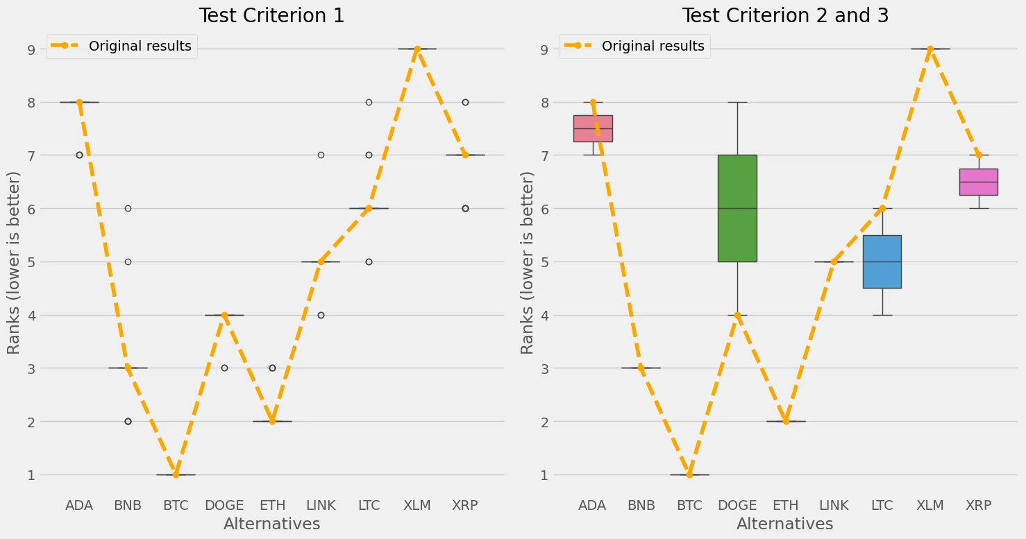
Test criterion 1 evaluates the stability of an MCDM method’s top-ranked alternative under minor degradations of non-optimal alternatives, which roughly attempts to detect rank reversals due to irrelevant changes.
Rank Invariant Checker, which will:
- Apply small degradations to each suboptimal alternative,
- Recompute the ranking each time
- Collect and compare all rankings.
This allows us to observe:
- How stable each alternative’s position is,
- Whether the top-ranked option remains consistent,
- How sensitive each alternative is to perturbations.
Test criterions 2 and 3
Test criterions 2 and 3 are closely connected in their goal of evaluating the internal consistency and robustness MCDMs via problem decomposition.
Test Criterion 2 (Transitivity): Ensures that transitivity holds across pairwise comparisons that is, if alternative A1 > A2, and A2 > A3, then A1> A3.
Test Criterion 3 (Recomposition Consistency): Builds a total ordering from pairwise relationships to recompose them into a complete global ranking for comparison against the original ranking.
class Transitivity Checker, that runs both tests secuentially and yields all the relevant details about the test criterions that were encountered in the process.
To verify that we made the right choice picking specific model, we’ll be using the TransitivityChecker.
- allow_missing_alternatives: desicion maker pipelines can sometimes return rankings with fewer alternatives than the original ones (using a pipeline that implements a filter, for example), which could cause issues in some partitions. This parameter allows for missing alternatives in a ranking to be added with a value of the maximum value of the ranking obtained + 1.
- max_ranks: limits the amount of rankings that can be constructed during the recomposition phase.
Results
- Test Criterion 2 Result: Indicates whether the method maintains transitivity across all pairwise comparisons
- Test Criterion 3 Result: Shows whether the recomposed ranking matches the original ranking
- Transitivity Break Rate: A normalized measure of how many transitivity violations exist relative to the theoretical maximum.
- Both criteria should return True, and the transitivity break rate should be 0, indicating robust decision-making consistency.
Case 1
Load dataset
we use dataset extracted from from historical time series cryptocurrencies. The nine available alternatives are based on the ranking of the 20 cryptocurrencies with the largest market capitalization calculated on the basis of circulating supply, according to information retrieved from Cryptocurrency Historical Prices” retrieved on July 21st, 2021, from there only the coins with complete data between October 9th, 2018 to July 6th of 2021.
  dm = datasets.load_van2021evaluation(windows_size=7)
  matrix = pd.DataFrame(dm.matrix).reset_index()
  matrix
| Alternatives | xRV | sRV | xVV | sVV | xR2 | xm |
|---|---|---|---|---|---|---|
| ADA | 0.029 | 0.156 | 8.14E+09 | 1.59E+10 | 0.312 | 1.82E-11 |
| BNB | 0.033 | 0.167 | 6.14E+09 | 1.12E+10 | 0.396 | 9.17E-09 |
| BTC | 0.015 | 0.097 | 2.1E+11 | 1.39E+11 | 0.281 | 1.25E-08 |
| DOGE | 0.057 | 0.399 | 8.29E+09 | 2.73E+10 | 0.327 | 1.46E-12 |
| ETH | 0.023 | 0.127 | 1E+11 | 8.05E+10 | 0.313 | 1.74E-09 |
| LINK | 0.04 | 0.179 | 6.71E+09 | 1.67E+10 | 0.319 | 1.58E-09 |
| LTC | 0.015 | 0.134 | 2.51E+10 | 1.73E+10 | 0.32 | 1.82E-09 |
| XLM | 0.013 | 0.176 | 4.16E+09 | 5.47E+09 | 0.321 | 1.88E-11 |
The Code
By calling, statistic.mdca_ranking we can generate MDCA with defined objective, weights, and what type MDCA algorithm that we want.
  dm, pipe, rank, final_rank = statistic.mdca_ranking(
                  main_data, objectives:list=[], weights:list=[], alt:str='', type:str="simple", is_plot=True, threshold=[0.65,0.35], non_dominated=False, target_sum='both')
This function requires the following parameters:
- main_data (
dataframe): Data Input - objectives (
list): List of objective with max min value. - weights (
list): List of weight value between 0 - 1. - alt (
str): name for each row or alternative. - type (
str): Type of MDCA algorithm. - is_plot (
boolean): to show plot for MDCA algorithm. - threshold (
list): list of threshold for electra algorithm. - non_dominated (
boolean): filter out for non-dominated row or alternative. - target_sum (
str): calculate weight value with 3 type of calculationmatrix,weights,both.
The result
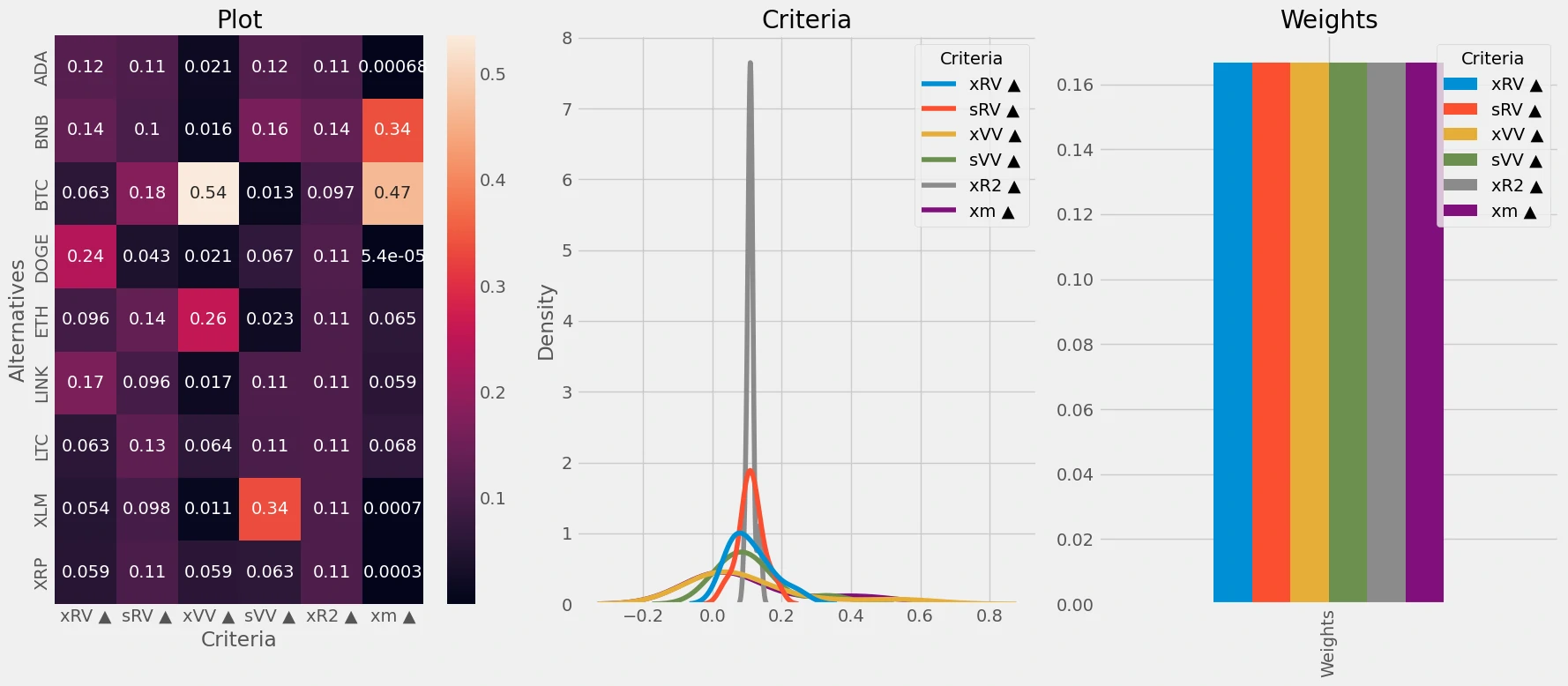
| rank | name | score |
|---|---|---|
| 8 | ADA | 0.079445 |
| 2 | BNB | 0.149775 |
| 1 | BTC | 0.225421 |
| 7 | DOGE | 0.080469 |
| 3 | ETH | 0.113801 |
| 5 | LINK | 0.09331 |
| 6 | LTC | 0.089931 |
| 4 | XLM | 0.101735 |
| 9 | XRP | 0.066114 |
Evaluation
statistic.mdca_evaluation(dm, rank, pipe, repeat=2, max_ranks=100)
  Transitivity Analysis Results:
  Test Criterion 2 (Transitivity): True
  Test Criterion 3 (Recomposition Consistency): False
  Transitivity Break Rate: 0.0000
Comparing
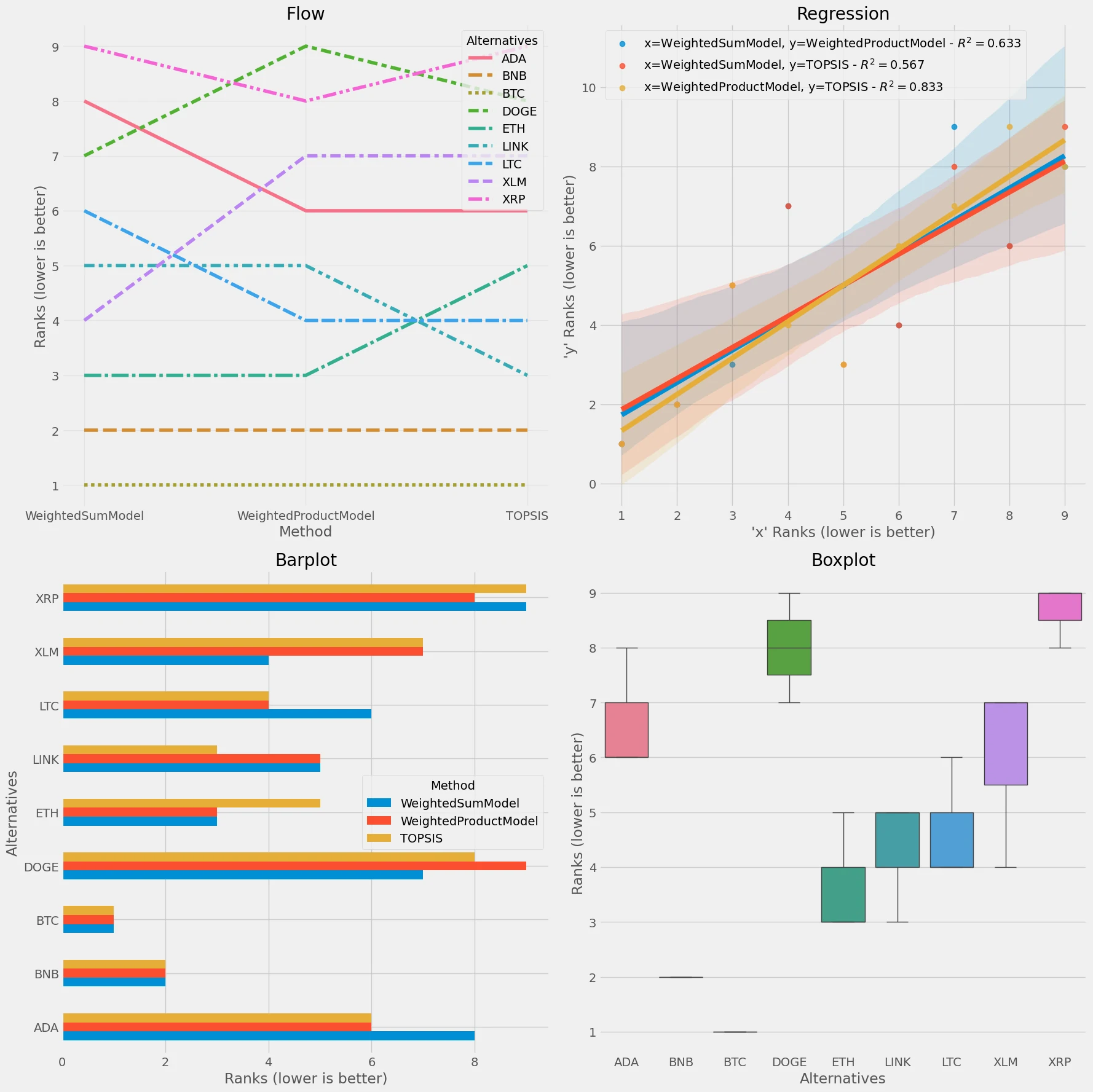
  rank_list, final_rank_list, final = statistic.mdca_comparing(
    ['sum','product','topsis'], matrix,
    objectives=objectives, weights=weights, alt='Alternatives',
    type="topsis", non_dominated=True, target_sum=['both','weights','weights']
  )
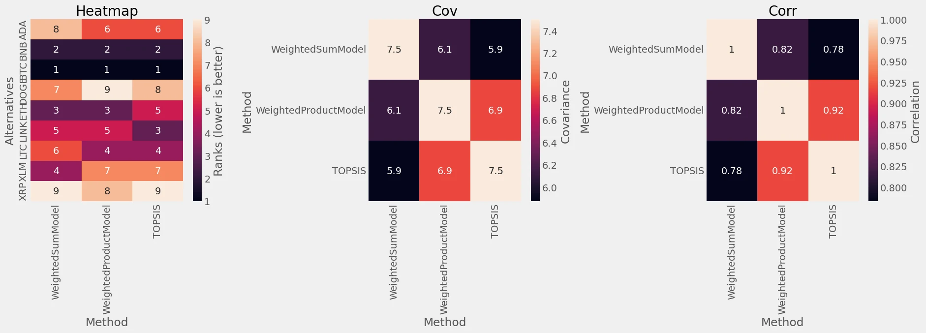
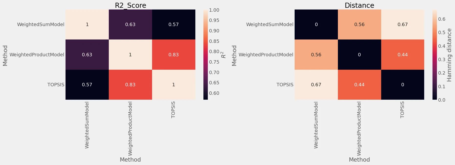
| Alternatives | WeightedSumModel | WeightedProductModel | TOPSIS |
|---|---|---|---|
| ADA | 8 | 6 | 6 |
| BNB | 2 | 2 | 2 |
| BTC | 1 | 1 | 1 |
| DOGE | 7 | 9 | 8 |
| ETH | 3 | 3 | 5 |
| LINK | 5 | 5 | 3 |
| LTC | 6 | 4 | 4 |
| XLM | 4 | 7 | 7 |
| XRP | 9 | 8 | 9 |
Case 2
Load dataset
we use Electric Vehicles dataset with some parameters to define EV performance.
  df = pd.read_csv('vans.csv')
  matrix
| code | name | manufacturer | carryfying capacity | max velocity | travel range | engine power | engine torque | battery charging 100% | battery charging 80% | battery capacity | price |
|---|---|---|---|---|---|---|---|---|---|---|---|
| A1 | EVI MD | Electric Vehicles International | 3000 | 96 | 145 | 200 | 610 | 10 | 120 | 99 | 120 |
| A2 | EVI Walk-In Van | Electric Vehicles International/Freightliner Custom Chassis Corp. | 2000 | 100 | 145 | 200 | 610 | 10 | 120 | 99 | 90 |
| A3 | e-NV200+ | Nissan | 705 | 120 | 170 | 80 | 270 | 4 | 30 | 24 | 25 |
| A4 | e-Wolf Omega 0.7 | e-Wolf | 613 | 140 | 180 | 140 | 400 | 8 | 40 | 24.2 | 50 |
| A5 | Minicab-MiEV Truck | Mitsubishi Motors Corp. | 350 | 100 | 110 | 30 | 196 | 4.5 | 15 | 10.5 | 12.9 |
| A6 | Mitsubishi Minicab-MiEV (10.5 kWh) | Mitsubishi Motors Corp. | 350 | 100 | 100 | 30 | 196 | 4.5 | 15 | 10.5 | 15.5 |
| A7 | Mitsubishi Minicab-MiEV (16kWh) | Mitsubishi Motors Corp. | 350 | 100 | 150 | 30 | 196 | 7 | 35 | 16 | 18.7 |
| A8 | Partner Panel Van | Peugeot | 635 | 110 | 170 | 49 | 200 | 8 | 35 | 22.5 | 31.5 |
| A9 | Phoenix Motorcars SUV | Phoenix Motorcars | 340 | 150 | 160 | 110 | 500 | 6 | 10 | 35 | 45 |
| A10 | Piaggio Porter electric-power | Piaggio Porter | 750 | 57 | 110 | 10 | 80 | 8 | 120 | 35 | 24.4 |
The Code
By calling, statistic.mdca_comparing_v2 we can generate MDCA with defined objective, weights, and what type MDCA algorithm that we want.
rank_score, rank = mdca_comparing_v2(type_list, main_data, objectives:list=[], weights=None, alt:str='', is_plot=False)
This function requires the following parameters:
- main_data (
dataframe): Data Input - objectives (
list): List of objective with max min value. - weights (
list): List of weight value between 0 - 1. - alt (
str): name for each row or alternative. - type_list (
list): List of MDCA algorithm. - is_plot (
boolean): to show plot for MDCA algorithm.
The result
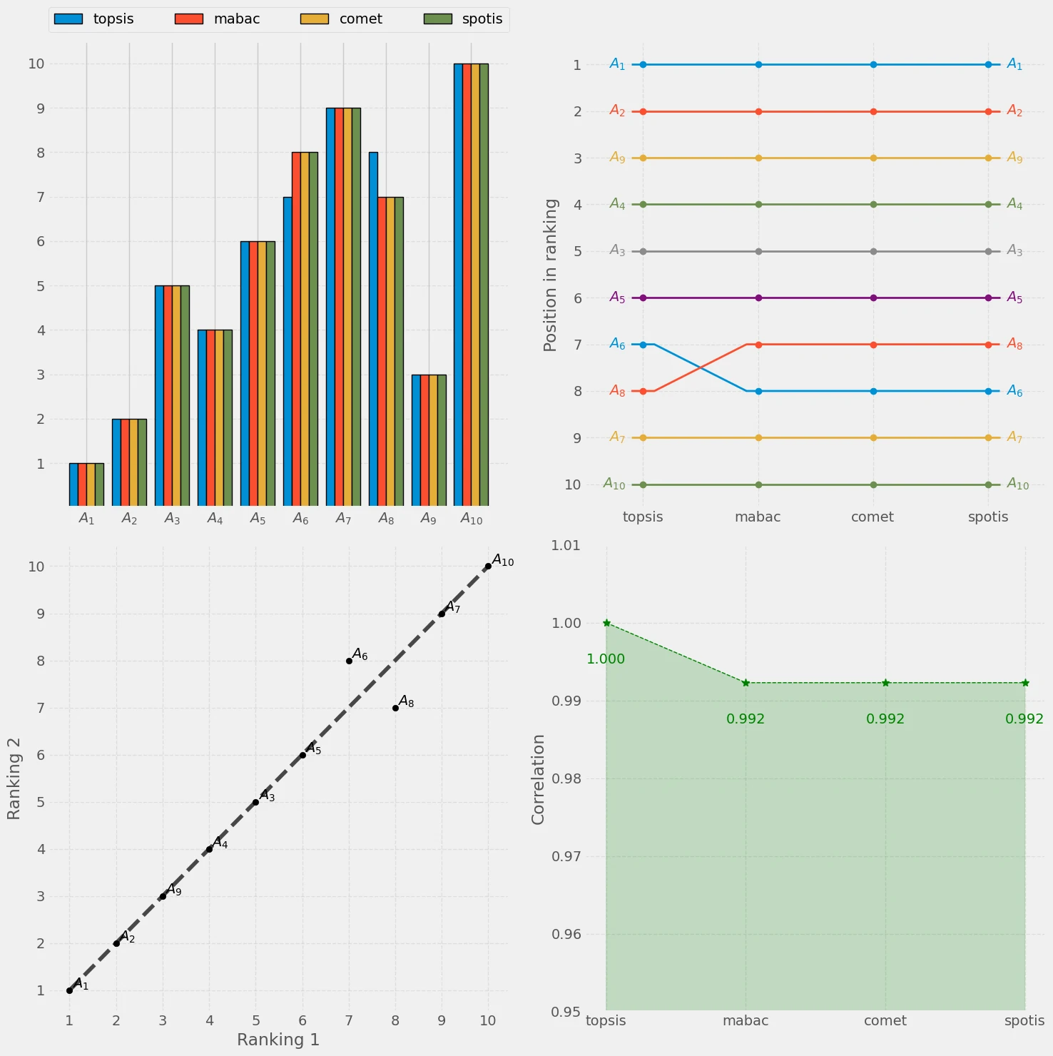
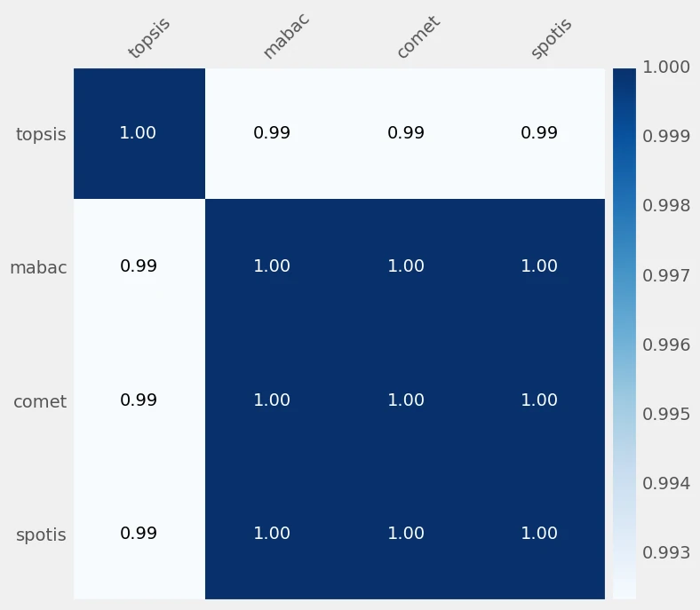
Rank Score
| topsis | mabac | comet | spotis | alternatives |
|---|---|---|---|---|
| 0.5762 | 0.2286 | 0.7459 | 0.368 | EVI MD |
| 0.5619 | 0.1993 | 0.6906 | 0.3973 | EVI Walk-In Van |
| 0.4593 | 0.0675 | 0.3961 | 0.5291 | e-NV200+ |
| 0.4641 | 0.0732 | 0.3991 | 0.5234 | e-Wolf Omega 0.7 |
| 0.4296 | -0.0129 | 0.282 | 0.6095 | Minicab-MiEV Truck |
| 0.4271 | -0.0178 | 0.2762 | 0.6144 | Mitsubishi Minicab-MiEV (10.5 kWh) |
| 0.3982 | -0.0489 | 0.2208 | 0.6455 | Mitsubishi Minicab-MiEV (16kWh) |
| 0.4117 | -0.016 | 0.2781 | 0.6126 | Partner Panel Van |
| 0.4981 | 0.1284 | 0.4969 | 0.4682 | Phoenix Motorcars SUV |
| 0.2997 | -0.1852 | 0.0765 | 0.7818 | Piaggio Porter electric-power |
Ranking
| topsis | mabac | comet | spotis | alternatives |
|---|---|---|---|---|
| 1 | 1 | 1 | 1 | EVI MD |
| 2 | 2 | 2 | 2 | EVI Walk-In Van |
| 5 | 5 | 5 | 5 | e-NV200+ |
| 4 | 4 | 4 | 4 | e-Wolf Omega 0.7 |
| 6 | 6 | 6 | 6 | Minicab-MiEV Truck |
| 7 | 8 | 8 | 8 | Mitsubishi Minicab-MiEV (10.5 kWh) |
| 9 | 9 | 9 | 9 | Mitsubishi Minicab-MiEV (16kWh) |
| 8 | 7 | 7 | 7 | Partner Panel Van |
| 3 | 3 | 3 | 3 | Phoenix Motorcars SUV |
| 10 | 10 | 10 | 10 | Piaggio Porter electric-power |