Detecting Palm Trees using Deep Learning
Computer Vision
Palm Trees
Introduction
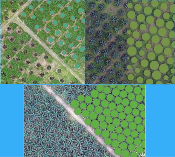
Palm trees are important economic crops in many tropical countries. The number of palm trees in a plantation area is important information for predicting the yield of palm oil, monitoring the growing situation of palm trees and maximizing their productivity, etc.
Traditionally, the counting of trees was done using physical survey or visual interpretation of imagery. An alternative technique is deep learning which can reduce time, resources and costs involved in such tasks. This technique can also be highly accurate.
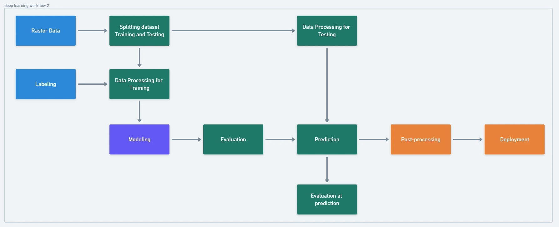
Simple Deep Learning Development
Model description
- Input: This model is expected to perform with aerial imagery (5 - 15 cm resolution)
- Applicable geographies: This model is expected to work all over the world.
- Architecture: This model uses the
SAMLoRAmodel architecture implemented in ArcGIS API for Python. - Accuracy Metrics: This model has an average precision score of 0.90.
Preprocessing
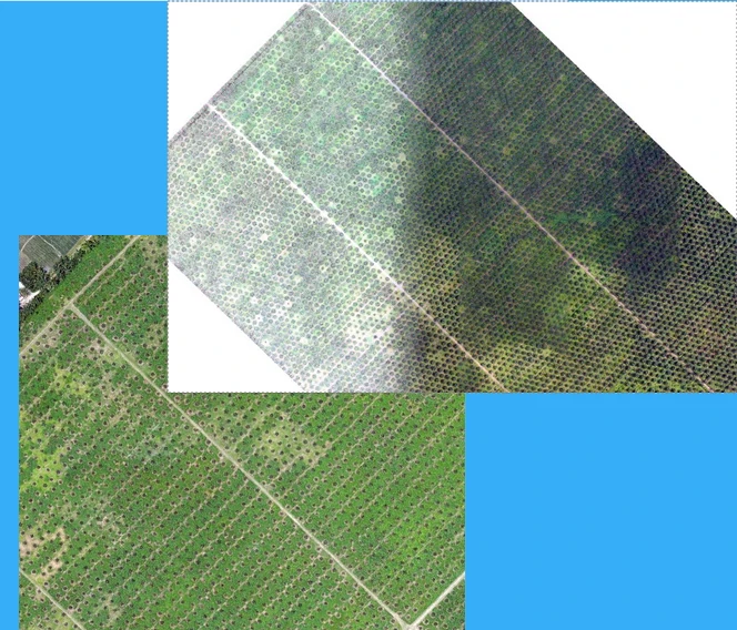
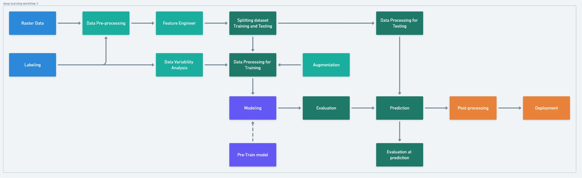
Data quality of input data sets the ceiling for model performance. Preprocessing ensures our imagery is clean, consistent, and focused before training. Especially important when training on remote sensing imagery with varying acquisition conditions.
Examples:
- Normalize imagery (e.g., same resolution, scale, CRS).
- Remove irrelevant information (clouds, shadows, no-data areas).
- Clip and tile imagery for manageable input sizes (e.g., 256x256, 512x512).
- Apply feature engineering, such as smoothing, sharpening, or color corrections if needed.
- Radiometric correction
Feature Engineering – Elevating Model Understanding
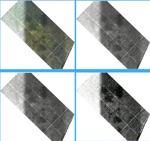
Raw RGB imagery often isn’t enough. Feature engineering gives our model more context. By incorporating additional bands, we help the model focus on traits that separate we target object from its background. More meaningful features lead to more onfident predictions.
Examples:
- Adding vegetation indices or terrain-derived layers (NDVI, GNDVI as extra channels) to better highlight objects like trees, water, or buildings.
- Derive texture metrics using focal statistics, histogram equalization, clustering pixel image or edge detection.
- Add non-visual band (e.g. NIR)
2 Geoprocessing tools that we can use in ArcGIS Pro namely:
-
Iso Cluster Unsupervised Classification: Performs unsupervised classification on a series of input raster bands using the Iso Cluster and Maximum Likelihood Classification tools.
-
Segment Mean Shift: Groups adjacent pixels that have similar spectral characteristics into segments. Each output raster from above tools can be combine with original raster using
CompositeBandstools.
Choosing the Right Model Type
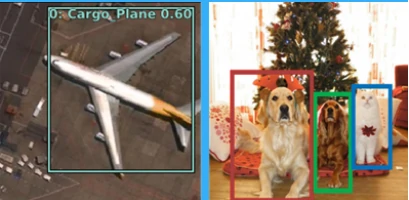
- Object detection
Object detection is the process of locating features in an image. The model be able to detect the location of different objects. This process typically involves drawing a bounding box around the features of interest.
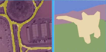
- Semantic segmentation
Semantic segmentation occurs when each pixel in an image is classified as belonging to a class. In GIS, this is often referred to as pixel classification, image segmentation, or image classification.
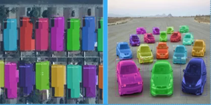
- Instance segmentation
Instance segmentation is a more precise object detection method in which the boundary of each object instance is drawn. This type of deep learning application is also known as object segmentation.
Different deep learning tasks solve different problems. Choosing the right model type ensures we’re solving ours efficiently. ArcGIS supports various deep learning models—U-Net, Mask R-CNN, and YOLO—each with strengths depending on our task. Choosing the right backbone, like ResNet or MobileNet, lets we balance performance with processing speed.
Examples:
- Object Detection (YOLO, Faster R-CNN): Output = bounding boxes.
- Semantic Segmentation (U-Net, DeepLab): Output = class per pixel.
- Instance Segmentation (Mask R-CNN): Output = individual object masks.
In example for each model type:
- Object detection
- Semantic segmentation
- Instance segmentation
Training Data Variability Analysis
Before labeling or training, we need to visually analyze the diversity of the objects and environments across the imagery. This helps ensure the model sees enough variation to generalize.
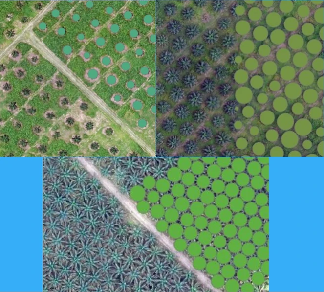
Examples:
- Examine imagery across regions and time
- Identify intra-class variability: object size, shape, orientation, illumination, background complexity.
- Palm trees may look different in highland vs lowland terrain or on different soil types.
- Use Export Training Data for Deep Learning to sample image chips and view in a mosaic.
Model Limitations & Failure Zones
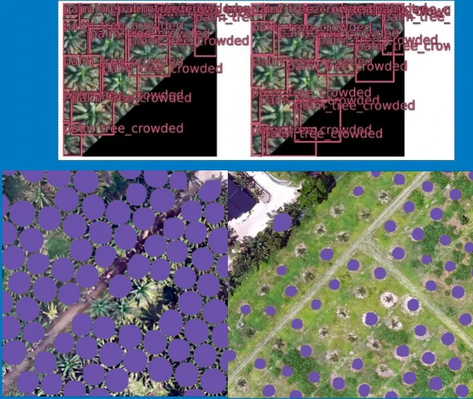
Even with strong training, deep learning models can fail—especially in unseen conditions. Knowing where and why this happens is key to improvement.
 20
20
Examples:
- Causes: unseen backgrounds, poor lighting, extreme object deformation.
- Visualize errors using prediction overlays and confidence maps.
- Flag and relabel failure zones for retraining (closed feedback loop) and to guide future labeling.
Final and Complete Deep Learning Development
How to measure the detected object?
-
Using Minimum Bounding Geometry Creates a feature class containing polygons which represent a specified minimum bounding geometry enclosing each input feature or each group of input features.
-
Using custom script:
- Calculate boundary area coverage
- Measure the center point of boundary area
- Measure the radius from the area (radius = math.sqrt(area / pi))
- Utilize buffer with center point and radius to create circle
Final Thoughts
By applying structured practices—clear labeling, preprocessing, feature engineering, and leveraging transfer learning—we turn GIS deep learning from experimental to production-ready. The ArcGIS ecosystem gives us the full pipeline to do this efficiently.
Deep learning in GIS is both art and science. It takes thoughtful preparation, the right tooling in ArcGIS, and iterative refinement. With these principles, your model’s performance will go beyond expectations.